Wall-Function Treatment
Continuing from the post about derivation of the logarithmic region of the turbulent boundary layer, this post aims to elaborate on how CFD codes compute the wall shear stress for various scenarios of mesh refinement.
Note that this is just a basic introduction into wall functions. Modern CFD codes use advanced wall functions such as the Spalding Function (named Standard Wall Functions in ANSYS Fluent). Also the concept of \(y^+\) and wall-functions apply to only turbulent boundary layers, and not its laminar counterparts.
Motivation for use
When a domain is discretised, generally speaking, the solution between the cells are interpolated in a linear fashion. Hence, regions where the solution variable changes rapidly (i.e., has a high gradient), a finer mesh setting is required to capture the solution in a piece-wise linear fashion.
One region where the solution variable has high gradient is the velocity near the wall, which also directly influences the wall shear-stress computation. Hence, ideally we need quite a fine mesh to capture the region near the wall, otherwise the solution is not resolved appropriately, as in images below.
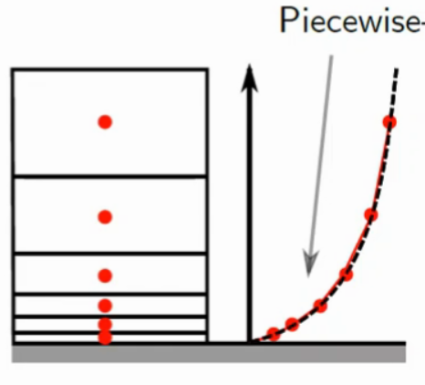 Refined mesh near the wall to capture the solution
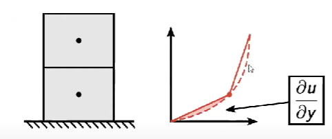 A coarse mesh fails to capture the solution properly
This is a huge problem in CFD, since all of the impact on the entire fluid domain is because of the presence of the walls and the boundary layers, hence it is crucial that the solution is captured properly.
But sometimes, say for high Re flows, the boundary layer is much smaller, making the requirement of the mesh refinement also very fine, the orders of \(y^+\) of 1 requires very fine mesh which makes the computation time also very high, which may not be affordable or feasible in many cases. So, there needs to be a way to have a coarse mesh but still have an accurate solution, and this naturally involves a non-linear interpolation between the first cell and the wall as in the below image. This involves the utilisation of the wall-functions
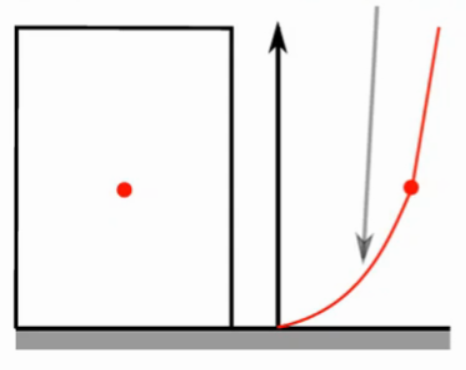 Non-linear interpolation using wall functions
Logarithmic Dependence of velocity profile with \(y^+\)
Recall that the variation of velocity profile in a turbulent boundary layer is linear at first, and then changes to logarithmic as the solution progresses from the viscous sublayer to the logarithmic region. This relation could be utilised for the wall-functions.
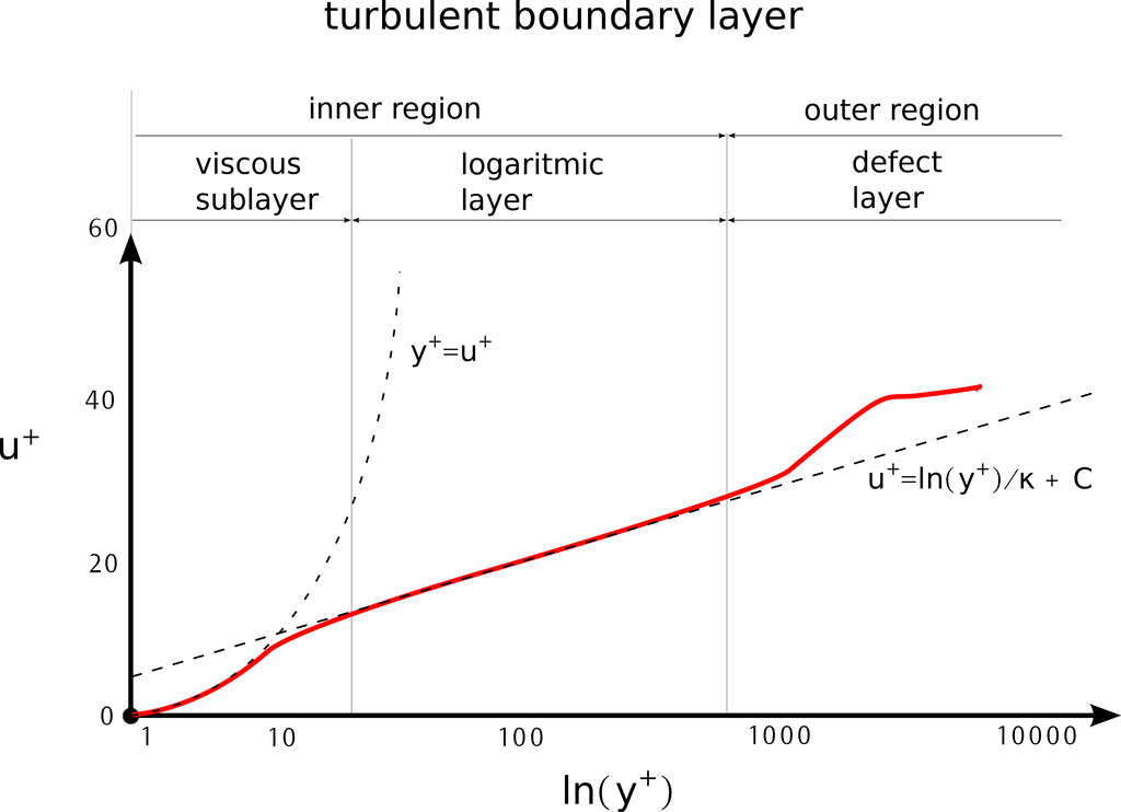 Velocity profile variation with y+
To find the intersection point between the two functions:
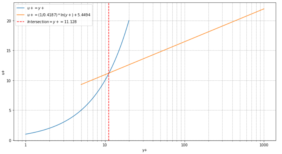 Intersection point of the two functions
Mathematically, this can be expressed as
\[\begin{equation} U^+ = \begin{cases} y^+ & y^+ < 11.13 \\ \frac{1}{\kappa}\ln y^+ + B & y^+ > 11.13 \end{cases} \label{eq:1} \end{equation}\]Wall Viscosity
This mathematical expression can be used for formulating a basic wall function. Near the wall, the shear stress only has the laminar component and no turbulent component, the latter of which arises from the fluctuating component of velocities. It is given by:
\[\begin{equation} \tau_w = \mu \frac{\mathrm{\partial}U}{\mathrm{\partial}y} \label{eq:2} \end{equation}\]Numerically, when no wall functions are used, this expresses condenses to:
\[\tau_w = \mu \frac{U_p}{y_p}\]where \(y_p\) is the height of the first cell centroid from the wall, while \(U_p\) is the velocity in that cell. This is the form in which we want the CFD code to compute the wall shear stress. Hence, we define the viscosity here as “wall viscosity, it will be seen why in next sections.
\[\begin{equation} \tau_w = \mu_w \frac{U_p}{y_p} \label{eq:3} \end{equation}\]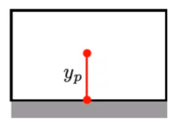 First cell centroid distance from wall
Before going to the wall functions, the LHS of \eqref{eq:1} is modified slightly:
\[\begin{equation} U^+ = \frac{U_p}{u_{\tau}} = \frac{U_p u_{\tau}}{u_{\tau}^2} = \frac{U_p u_{\tau} \rho}{\tau_w} \label{eq:4} \end{equation}\]where \(u_{\tau}\) is the “Friction Velocity”.
To use the wall function from the expression given by \eqref{eq:1}, we have two scenarios:
Different regions of wall function computation
First cell within \(y^+ < 11.13\)
If the first cell is placed within this range, the first expression from \eqref{eq:1} is used for calculating the wall shear stress. From equations \eqref{eq:1} and \eqref{eq:4}:
\[\frac{U_p u_{\tau} \rho}{\tau_w} = y^+\] \[\tau_w = \frac{U_p u_{\tau} \rho}{y^+} = \frac{U_p u_{\tau} \rho}{\frac{\rho y_p u_{\tau}}{\mu}} = \mu \frac{U_p}{y_p}\]Which is of the same form as \eqref{eq:3}. Hence for this region of \(y^+\), \(\mu_w = \mu\), or the viscosity of the fluid itself.
This similarity arises because both the numerical interpolation between the cell centroids and the natural variation of velocity profile with the cell distance from wall are linear.
First cell in \(y^+ > 11.13\)
In case mesh refinement is taking a lot of computational resources, and the first cell lies beyond the \(y^+\) of 11.13, from equations \eqref{eq:1} and \eqref{eq:4}:
\[\frac{U_p u_{\tau} \rho}{\tau_w} = \frac{1}{\kappa}\ln y^+ + B\] \[\tau_w = \frac{U_p u_{\tau} \rho}{\frac{1}{\kappa}\ln y^+ + B}\]Comparing this with the form given by \eqref{eq:3},
\[\mu_w \frac{U_p}{y_p} = \frac{U_p u_{\tau} \rho}{\frac{1}{\kappa}\ln y^+ + B}\] \[\mu_w = \frac{y_p u_{\tau} \rho}{\frac{1}{\kappa}\ln y^+ + B}\]Wall Function
Consolidating, the wall function approach as per the basic logarithmic function derived as per \eqref{eq:1} involves utilisation of a “wall viscosity” which takes on a different value based on where the first cell is usually placed.
- If the mesh is refined, the fluid viscosity is used as the wall viscosity. Or, in other words, a linear velocity profile w.r.t \(y^+\) is used to compute the wall shear stress
- If the mesh is coarse (in case mesh refinement near the wall is not an option), the logarithmic wall function is used for thewall viscosity, which is used to compute the wall shear stress.
The wall viscosity is mathematicall hence given as:
\[\mu_w = \begin{cases} \mu & y^+ < 11.13 \\ \frac{y_p u_{\tau} \rho}{\frac{1}{\kappa}\ln y^+ + B} & y^+ > 11.13 \end{cases}\]Points to Note
- For this wall function to produce accurate results, it has to be noted that the velocity profile varies logarithmically only in the overlapping log-layer, which could be thin for low Reynolds number flows, the upper bound of which could be as low as \(y^+\) of 150. Hence placement of the first cell within this region is crucial, otherwise it could use the logarithmic function even when the first cell may be in the outer layer of the boundary layer
- For high Reynolds number flows, the upper bound of the overlapping log-layer could be in 100s of \(y^+\), hence this problem is not present.
- Another thing to note is that the experimental correlation of \(U^+\) and \(y^+\) (quite closely followed by the Spalding Function) does not match with the expression given in \eqref{eq:1} between the \(y^+\) values of 5 and 40, approximately. Hence, if the first cell is placed within this region (often called the Buffer Layer), this particular wall function may not give accurate results
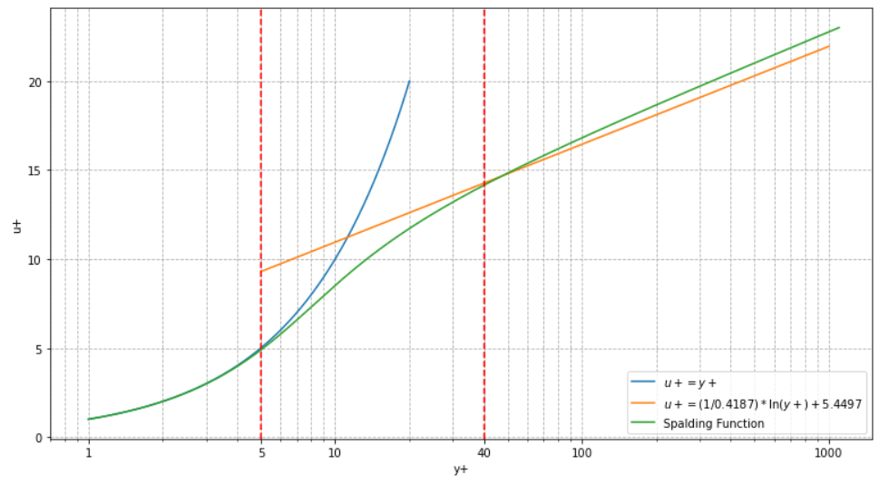 Spalding Function
- But nowadays, the spalding function is the more widely used wall function, which closely follows the experimental correlation between \(U^+\) and \(y^+\), which is evidentally robust enough to handle the anomaly of placing the first cell in the buffer layer. It is a single function unlike the piecewise varying function used for this post, and is given by: