Delay and Sum Beamforming - 1
Continuing from my investigations and studies in Signal Processing, the next technique I want to explore is Spatial Filtering. Particularly, Beamforming.
In many applications, particularly Automotive External Aero-Acoustics (this is an area of interest of mine as a CFD engineer dabbling in Aero-dynamics/acoustics), it is crucial to know the areas where broadband acoustic noise generation is high. For this, some sort of directionality is important as to understand from where the noise or sound is coming from. Beamforming is one such technique which uses an array of microphones to arrive at direction of noise signals received by the array.
In this post, we will see an intuitive approach to understand this process, and then expand to a complicated, industrial setup ready for deployment.
Temporal Beamforming
The Beamforming technique involves several signal processing operations in both the time and frequency domain, but for a fundamental level understanding, we will first look into the temporal processing with a simple 3-mic array [2].
Take the case of a simple three microphone array arranged in a line. We will pass a signal wave at an angle to this setup, in the same plane of this array, as in figure below:
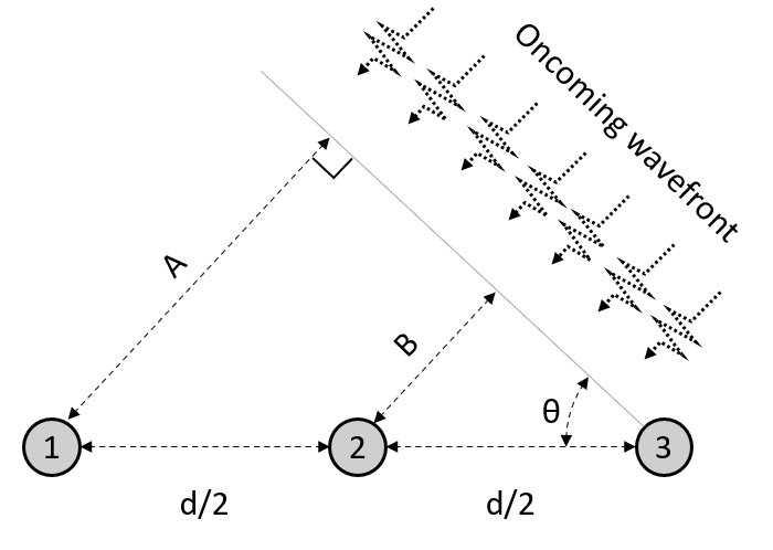 A Simple 3-mic setup with a sample oncoming wave
In this case, the recording received by mics 1 and 2 are delayed w.r.t mic 3 due to their relative orientation with respect to the incoming wave. To be precise, the time delay in the signal received by mic 1 and mic 2 is (considering a speed of the signal as $c_0$:
\[td_1 = \frac{A}{c_0}, \quad td_2 = \frac{B}{c_0}\] \[td_1 = \frac{d\mathbf{sin\theta}}{c_0}, \quad td_2 = \frac{d\mathbf{sin\theta}}{2c_0}, \quad td_3 = 0\]And subsequently, the signals received by the mics with respect to mic 3 ( $s_3(t) = s(t)$ ):
\[s_2(t) = s\left( t - td_2 \right), \quad s_1(t) = s\left( t - td_1 \right)\]Let us understand this with an example. Say take a case of a sinusoidal wave, 500Hz frequency and incident on the array at an angle of $\theta =$ 60°. In that case, by considering the above understanding of time delays, the signals from each mic overlapped look like this:
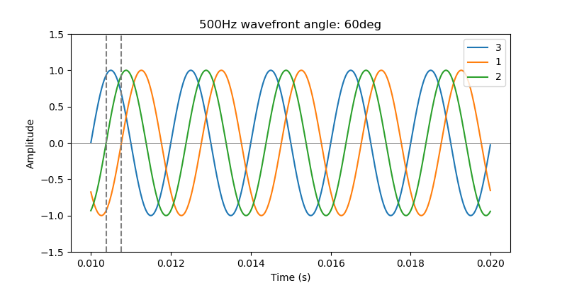 Angled Signal onto the 3-mic array setup
Notice the delay in the mics 1 and 2. The exact time delays are calculated as per the aforementioned definitions. Now, the actual recording of the array is the combined recording of each of the 3 mics for all time $t$.
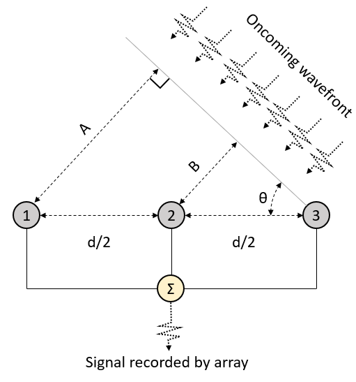 Recording of the array
In that case, for this example:
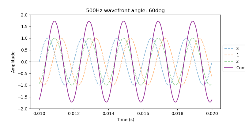 Array recording of the angled signal
Naturally, let us try the response now for various different angles of $\theta$. Intuitively, understand this as moving the array such that any given signal wavefront makes an angle $\theta$ with the setup.
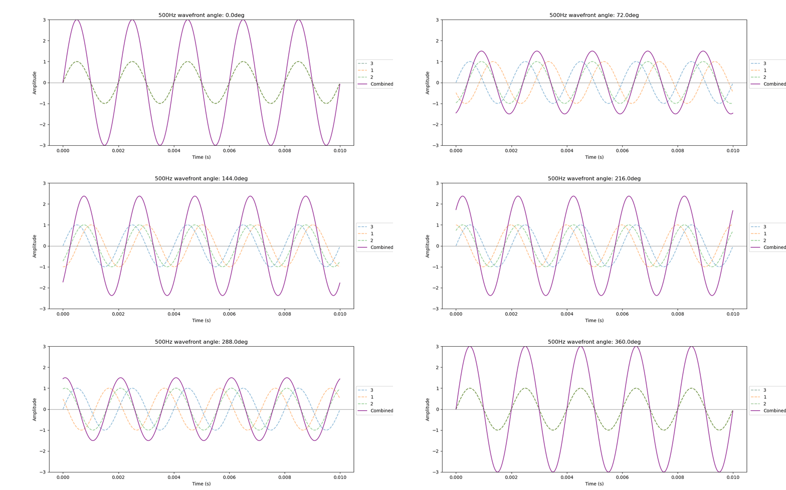 Array recording of the angled signal at various thetas
As expected, the response is maximum when the 3 recorded signals are in-phase, and hence add up constructively. This happens only when the signal is incident perpendicular to the array setup, such that there is no difference or time delay of any microphone with respect to each other.
In other words, the response of the array is maximum when you place the array such that it is aligned constructively ($\theta = 0$) with the incident wavefront.
In a way, very crudely, the array setup is helping us identify the region of noise. But this still needs some fine tuning, since as per the above understanding, we still need to move the setup like some kind of metal detector, to understand the exact direction of noise source.
Steering
Let us slightly shift perspectives here. Say a wave is coming at an angle $\theta =$ 60° which is yet unknown to the 3-mic array. As an experimental setup, it will only be able to see individual microphone recordings and the final aggregate response from the three mics. They are plot below:
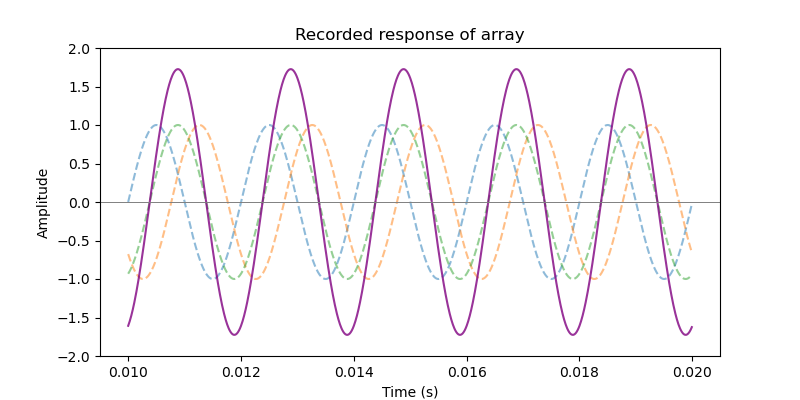 Array response
The above array will contain some time delays for mics 1 and 2 which are unknown to us [1], since $\theta$ is unknown. We shall call them:
\[td_{1actual} = \frac{d\mathbf{sin\theta_0}}{c_0}, \quad td_{2actual} = \frac{d\mathbf{sin\theta_0}}{2c_0}\]The corresponding signals recorded in mics 1 and 2 are hence:
\[s_2(t) = s\left( t - td_{2actual} \right), \quad s_1(t) = s\left( t - td_{1actual} \right)\]Which means, the two signals in mics 1 and 2 are phase-shifted/delayed by $td_{1actual}$ and $td_{2actual}$ seconds respectively, thus leading to a less-than-maximum response of the array.
Now, what if, we individually subtract these time delays from each mic? We take back the phase-shifted / delayed signals to the original wave, such that all the three mics now add up constructively. The signals would then look like:
\[s_2(t) = s\left( t - td_{2actual} + td_{2actual}\right) = s(t), \quad s_1(t) = s\left( t - td_{1actual} + td_{1actual} \right) = s(t)\]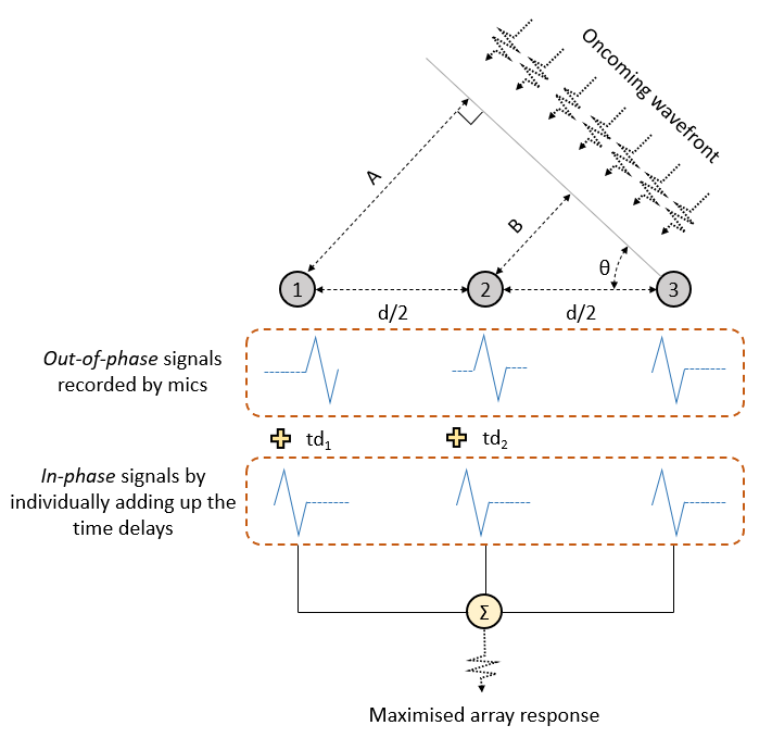 Individual time delays applied to mics 1 and 2
These processed signals, when added up, will give a completely in-phase signal between the three mics, and hence a maximised response. The only problem with this technique is, $\theta$ is unknown to us, and hence also $td_{1actual}$ and $td_{2actual}$. But, this is not a major issue. We shall simply iterate over various values $\theta$ for this.
To understand, let us assume a value of $\theta$. Say, $\theta_0$. Based on this assumption, we shall treat the original signals by recovering the time delays for mics 1 and 2 as mentioned above. Let the time delays for this assumed $\theta_0$ be $td_1$ and $td_2$ for mics 1 and 2 respectively. We know that the original signals are:
\[s_2(t) = s\left( t - td_{2actual} \right), \quad s_1(t) = s\left( t - td_{1actual} \right)\]Now, recovering the time-delays for $\theta_0$:
\[s_2(t) = s\left( t - td_{2actual} + td_{2}\right), \quad s_1(t) = s\left( t - td_{1actual} + td_{1} \right)\]The above array response is maximum when $td_{1} = td_{1actual}$ and $td_{2} = td_{2actual}$, or, when $\theta_0 = \theta$. We will try to visualise this iteration.
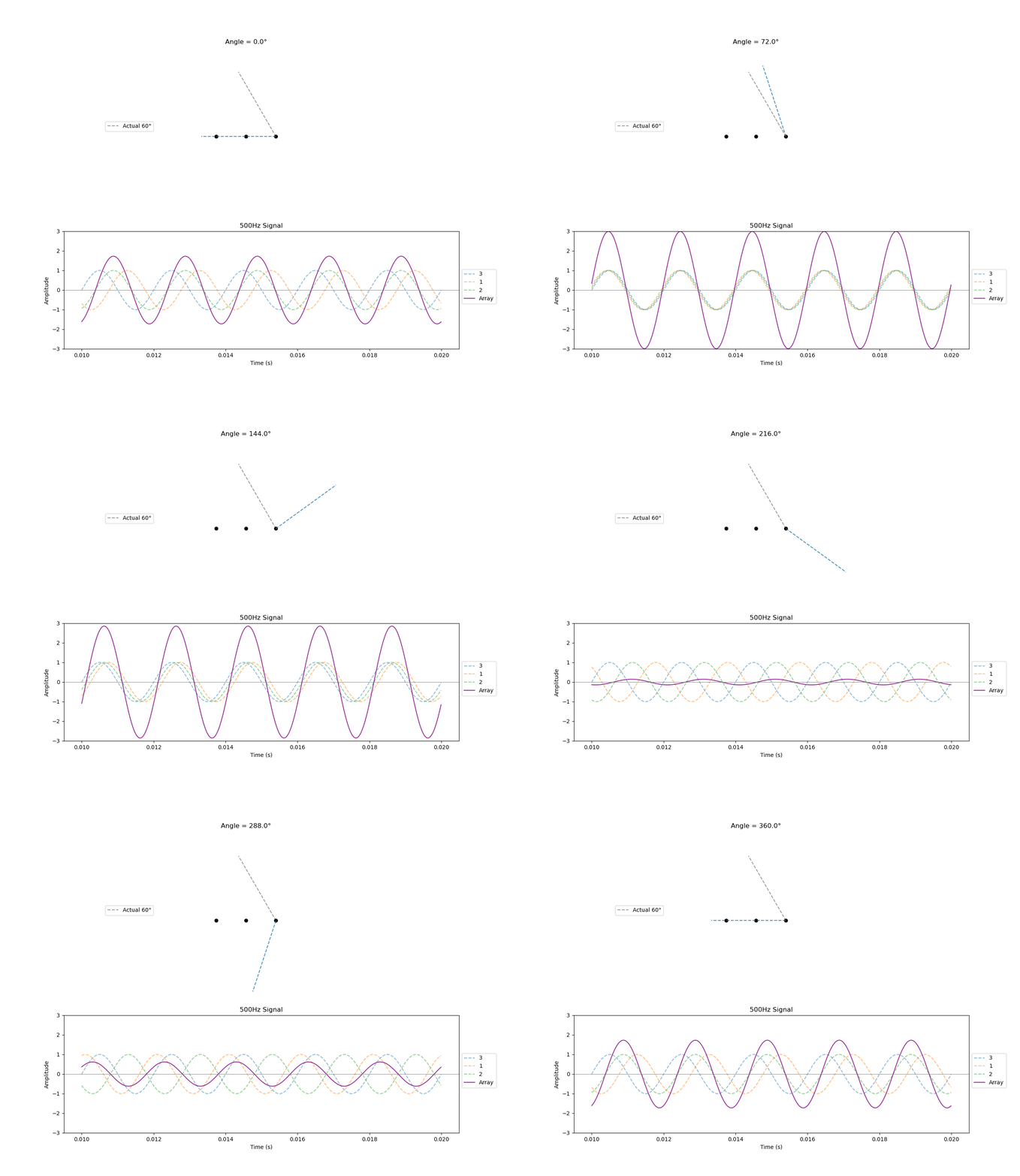 Iterating over various angles, and their responses
Please note that, in the above animation, the signals shown for mics 1 through 3 are merely for representation. It is not computed from the above process, and is also unknown to the iterator and the process in general.
Notice in the above animation, when iterating through the angles, it is similar to “steering” across various angles, searching for the actual angle of incidence of the signal. Hence, this process of iteration is also called Steering.
Now, let us plot the response of this array [3] at various angles.
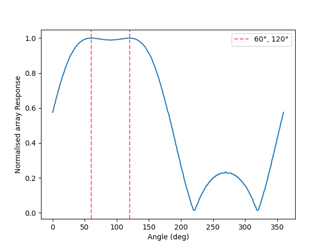 Array Responses vs Angles
And voila! This “Steering” technique is indeed predicting the angle of incidence accurately, providing the maximum array response at 60°, as the experiment originally started! One may wonder, why there is a peak at 120° as well. That is because of the one-dimensional nature setup of this array. At 120°, the array is exactly replicating the 60° scenario, but mirrored. This can be overcome by merely breaking the symmetry and introducing an L-shaped array, the “L” part being on the plane perpendicular to the screen.
The entirety of the above technique is the fundamentals of Delay-and-Sum Beamforming. Now, we shall explore further by introducing composite waves into the scenario. After that, we shall also pass multiple signals from different directions to test the performance of this beamformer array setup.
Composite Waves
Consider a composite wave comprising of 2 individual signal components of frequency and amplitudes (500Hz, 1) and (290Hz, 1.3) respectively, both having the same phase.
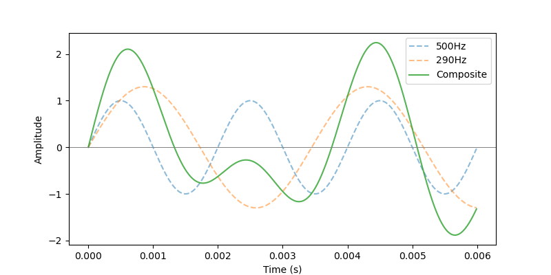 Composite wave example
Let us send this wave at an incident angle of $\theta$ = 55° with respect to the beamformer array. The recordings at each of the mics and the overall array aggregate is plot below.
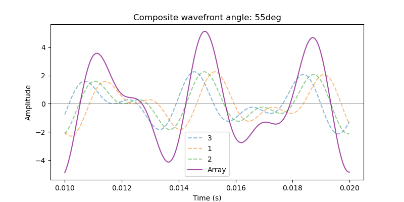 Composite wave actual Recordings
Do note that, as before, the angle itself is not known to the beamformer. Now, we shall check if the beamformer array is able to predict the angle of incidence accurately regardless of whether the signal passed is a single-frequency signal or multi-frequency composite. The Steering iterator is shown below:
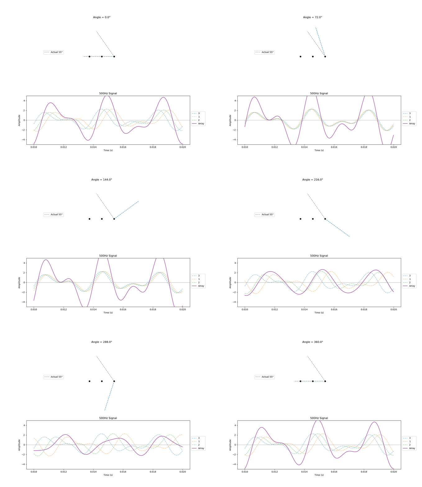 Steering of Composite wave example
In this case, when the “recording” of this Steering process matches with the actual aggregate recording of the array as plot before, the array response will be maximum. We can already get an idea of the maximised response when the steering approaches 55° (also notice that each mic recording is completely in phase at that angle). Anyway, the corresponding array responses for various angles are plot below:
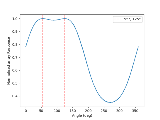 Array Responses vs Angles: composite signal example
The beamformer is still able to predict correctly the incident angle of the composite wave! Again, the same issue with 1D linear array is present due to the symmetry. Now let us explore another case, where I shall pass two monotone signals from two different angles.
Monotone signals from different direrctions
Consider this example of two monotone sine signals of equal amplitude, with frequencies 500Hz and 400Hz respectively, arriving at the array at angles 55° and 325° respectively. An angle of 325° just means the signal is arriving from the left (or bottom right, depends on how you look at it) side in the array setup as in the first figure of this post.
The individual signals are plot below, for each mic and as an array aggregate:
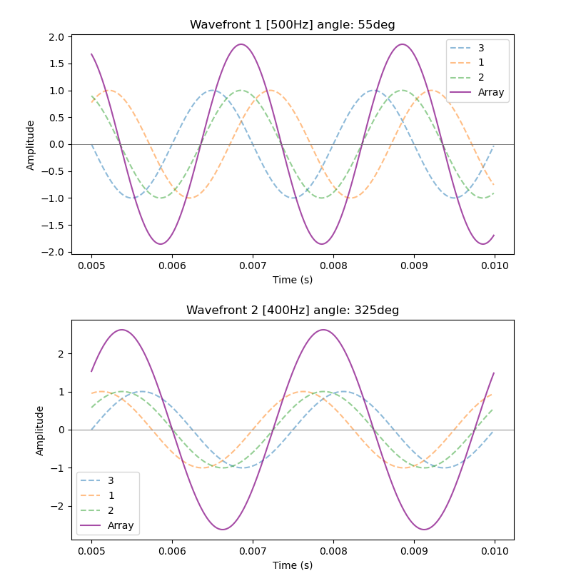 Multiple Monotone waves from different angles
Now again, this above information is not know to the array itself. What the array experiences is an aggregate of each of these signals. Below is plot what each mic “experiences” overlay with the contributions from each monotone signal unknown to the mics.
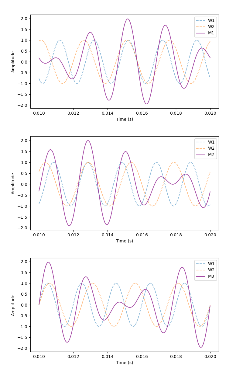 Multiple Monotone waves from different angles: Mic Recordings
The aggregate array recordings are, hence:
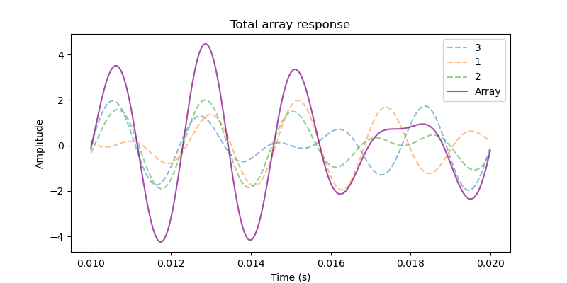 Multiple Monotone waves from different angles: Array recording
Now, we will repeat the steering process (with a goal to replicate the original/actual recorded signal):
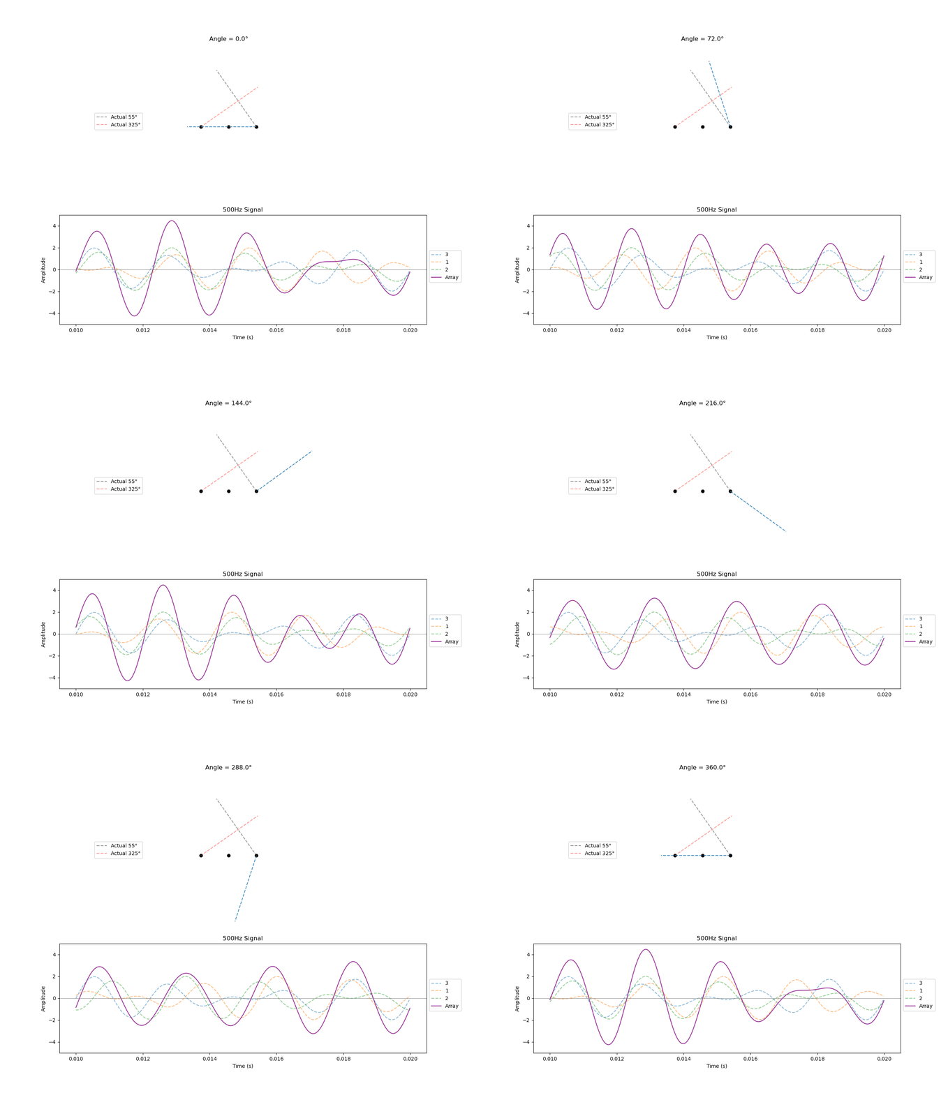 Steering
The array responses are plot below:
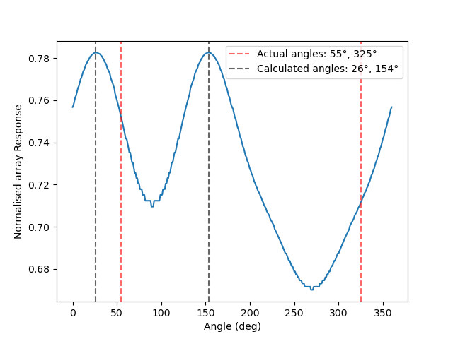 Array Responses vs Angles: different angles example
Well, unlike the previous two examples, it does not seem to be working in this case! But, it is not that something is wrong with the code, or methodology. It is perfectly correct, but this example highlights one of the limitations of the temporal beamforming.
For this scenario, we have 3 unknowns: Namely, the
- Angle
- Amplitude, and
- Phases of each of the signals. (In this case, the phase difference is inherently due to the difference in angles of incidence)
In the earlier case, it was not important to compute the amplitude and phases of each of the signals, since only one signal was arriving at the array setup. But in this case, due to the plurality of signals from multiple directions, it becomes important to distinguish each signal arriving at the array setup. For this, we need some kind of methodology to extract information of amplitude and phases of each of the signals from the composite signal which has been recorded by the array. It is something like extracting the different colour components from a mixed colour. Fortunately, we have a method for this,c alled the Fourier Transform.
The Fourier transform outputs information which contains the amplitude and phase of each individual component frequency present in a composite signal. [4]
Hence, the Fourier Transform converts a signal from the temporal domain, to information of amplitudes and phases in the frequency domain, thus splitting apart the signal to various individual frequencies.
Consequentially, this requires the Beamforming method (and also the Steering) to function in the frequency domain. While the idea remains the same, the mathematics takes on a more complex turn…
Anyway, the frequency-domain beamforming shall be discussed at length in the next post. [5]
Footnotes
[1] Looking at the graph, it may seem easy enough to compute the time delays in each mic, and the original statement may seem counter-intuitive. But once you deal with tens of mics, with very broadband signals ranging across many frequencies, then it becomes almost impossible and very time-consuming task to do this. Hence, the iterative approach is used as explained further.
[2] As one may wonder in their curiosity, what happens if you change the distance between the microphones, $d$? This directly leads to a concept called Spatial Aliasing, which introduces “ghost signals”, or prediction of signals from different directions which originally does not exist. To avoid this, there is a criteria called the Spatial-Nyquist criteria which is discussed at length here. The criteria says that, the distance between the microphones should be such that, it is less than half of the smallest (complete) wavelength (which corresponds to the maximum frequency component) present in the signal.
\[d \le \frac{\lambda_{min}}{2}\][3] The “reponse” from an array is defined here as the RMS value of the signal across time. This RMS is then normalised. Mathematically,
\[RMS_{array} = \sqrt{\frac{1}{T}\int_{0}^{T} x(t)^2dt}\]For a discrete signal,
\[RMS_{array} = \sqrt{\frac{1}{N}\sum_{n=1}^{N} x_n^2}\]This aggregate response of array is normalised w.r.t RMS response from each mic. For a given mic $i$, the RMS response is:
\[RMS_i (i=1,2,3) = \sqrt{\frac{1}{N}\sum_{n=1}^{N} x(i)_n^2}\]The normalised array response is thus:
\[NRMS_{array} = \frac{RMS_{array}}{\sum_{i=1}^{3}RMS_i}\][4] As to how this is done, is discussed in detail in the following posts:
[5] Further reading on DAS Beamformer:
- Part - 2 of Delay and Sum Beamforming: Understanding of the process in the frequency domain.
- Part - 3 of Delay and Sum Beamforming: Exploring an Engineering use-case DAS Beamformer.
[6] The codes for images and animations generated by self, and even further, are consolidated here.