Aliasing in Signal Processing
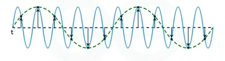
There are these famous videos in YT, where a helicopter is apparently flying with stationary blades. NO Rotation. This is called the “Strobe” effect, and it is a purely photographic phenomenon, where the frame rate of the camera exactly matches the rotation rate of the blades. This is, fundamentally, the concept behind Aliasing.
Yes, it is this simple. And very easy to visualise and intuitively understand in photo/video-graphy. But we will explore this concept in Digital Signal Processing.
Of course, since I have an unconventional, non-linear route to my learning in DSP, I come across the term “Aliasing” every now and then when reading on some other concepts.
Sampling
To first understand Aliasing, we have to go through Sampling.
Sampling is the process of converting a continuous real-world signal (analog) to a discrete time (digital) signal by taking “snapshots” (samples) at regular intervals. It is essential in signal processing to convert real-world sound, like voice or music in acoustics, into digital data that computers can process, store, and transmit.
Consider the below animation. A given wave (say, 20Hz) is sampled through at different intervals and a given “phase shift”. Notice for he various different sampling frequencies (SF), how the “sampled wave” (in orange) looks like:
- 10Hz SF: Captures all the zeroes (or peaks/troughs, depending on the phase-shift). And every “sample” lies exactly in the same spot of a single waveform of the 20Hz signal.
- The observation applies for 20Hz SF as well. When the sampling rate is equal to the signal wave itself, then the strobe effect as mentioned earlier comes into play.
- When you sample slightly slower (say, 19Hz SF), then you get a 1Hz wave owing to the difference between the signal frequency and the SF.
- When you sample slightly higher (21Hz SF), you sample the wave early: JUST BEFORE it finishes its cycle. And every time you sample, the point slightly moves backward in the 20Hz waveform, and hence you get a negative 1Hz wave.
Similarly, many such observations can be seen. So, capturing a f Hz wave at f Hz, is NOT a good idea. So what is the ideal Sampling Frequency for which you will be able to capture the information in the wave?
Notice that I used the word, “information”. That is, if we obtain just the peaks and troughs of the entire signal, then in effect we have information of the entire signal itself. The remaining data points are simply a sinusoidal interpolation. Our goal here is not to capture data points at very small intervals such that the entire wave form is captured in the sampling itself. By capturing just the extreme amplitudes, the remaining can be mathematically modeled / interpolated, thus saving a lot of space and computational time.
Either way, the minimum required sampling frequency would be by capturing two data points of the wave: the peak and the trough. That is, a sampling frequency of two times the signal frequency.
But notice in the below image again, that the peaks and troughs are not captured even at 40Hz, but only the zeroes!
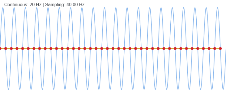 Sampling a 20Hz wave at 40Hz
Here we bring the concept of phase-shifting our sampling process. If the sampling starts from the “peak” of the first 20Hz waveform (i.e., the first quarter of the wave), then the sampled wave is:
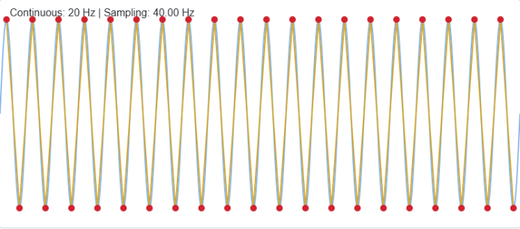 Sampling a 20Hz wave at 40Hz, phase-shifted by a quarter of waveform
As mentioned earlier, the entire wave information is captured in this sampling. This criteria, of the Sampling Frequency being atleast twice that of the signal frequency, is called the Nyquist-Shannon Criteria.
Consider this composite wave below:
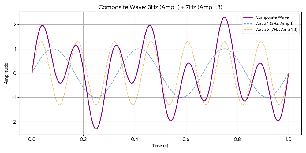 Composite wave with 3Hz and 7Hz
As an extension to the Nyquist-Shannon criteria: to capture any given wave, the global sampling rate must satisfy the fastest individual component (i.e., highest frequency) in the mix. The status of capturation of every frequency can be understood by treating each frequency independently present inside the composite wave. Take this example below:
For a Sampling Frequency of 14Hz (adjusting the phase to 0.25 in this case), each of the peaks and troughs of the composite wave is properly captured.
As a final experiment, we will also see sampling of a real-world broadband acoustic signal.
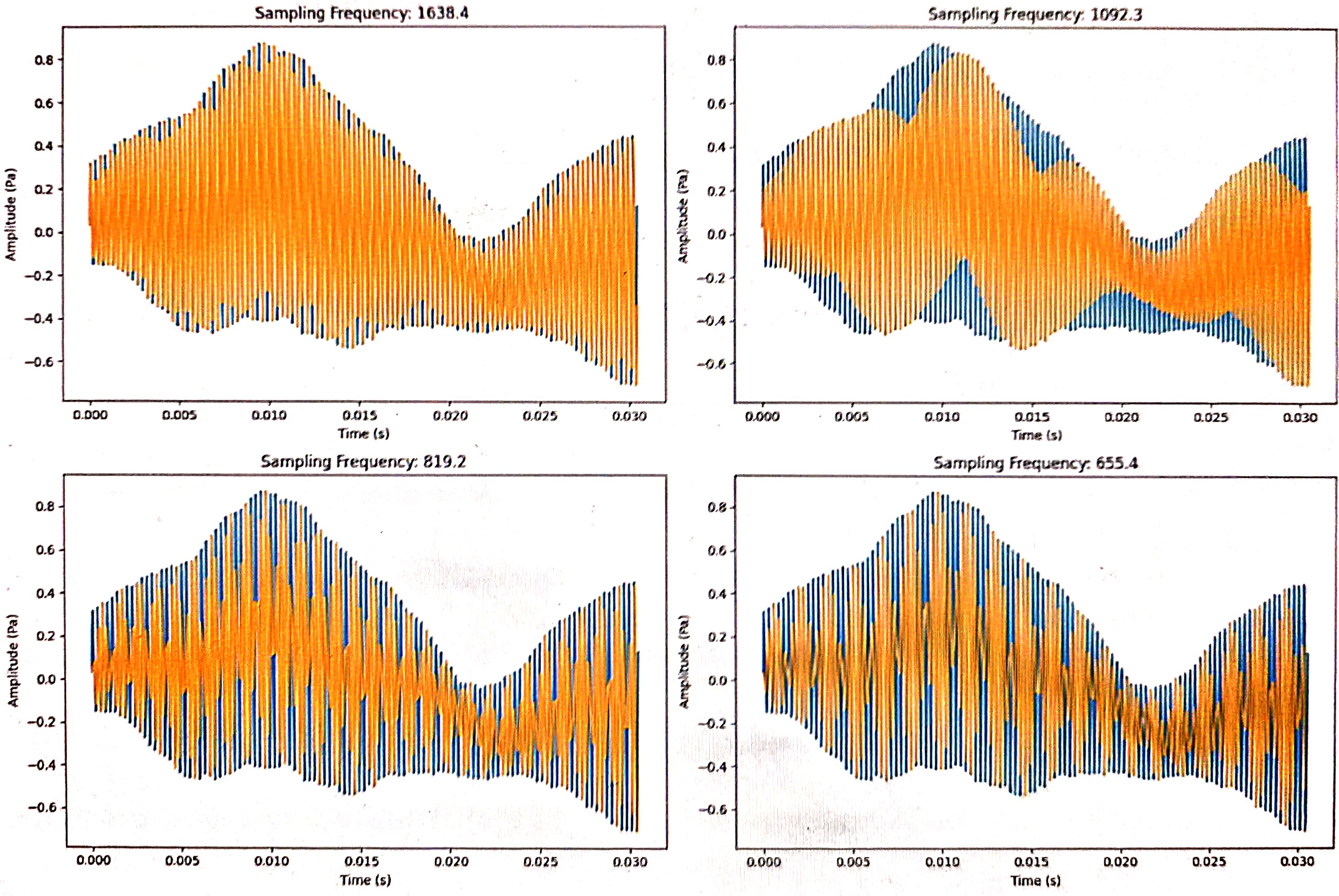 Acoustic Wave Sampling
To capture an acoustic wave, it is very critical as to what Sampling frequency we choose.
Now, this Nyquist-Shannon criteria is not a sufficient condition, but a necessary condition. As observed earlier, even with a sampling frequency of 2 x signal frequency, there can be “zero aliasing” (or any other kinds of aliasing for that matter). As a rule, the Sampling frequency is to be greater than twice the maximum frequency component present in a wave.
Hence it becomes critical as to how strategically we choose our sampling frequencies, especially considering the actual wave (especially in broadband signal scenarios) will be nothing like a pure sinusoidal wave.
Note: The reason it is mentioned that the sampling frequency should be “strictly greater than” is that at exactly 2xMaxFrequencyComponent, you aren’t capturing a “wave” - but just capturing two dots per cycle. If those dots hit the the zeroes or anything close to it, the sampled wave throws out a much dampened result, or even nothing.