Delay and Sum Beamforming - 2

• Introductory post on Delay and Sum Beamforming.
• Part 3 of DAS Beamforming, continuation of this post. Explaining a real-world engineering use-case Beamforming process.

Frequency-domain Beamforming

In the previous post (linked above), we concluded that the temporal beamforming technique was not good enough to identify the direction (in this specific case, the angles) from which signals are coming from if there are multiple signals from different directions. In that case, we have to separate out the information about the individual signal components from the aggregated recording which available to us in the test setup which is the three-mic array.

Let us continue with the problem we left off in the last post.

Two monotone sine signals of equal amplitude, with frequencies 500Hz and 400Hz respectively, arriving at the array at angles 55° and 325° respectively. An angle of 325° just means the signal is arriving from the left (or bottom right, depends on how you look at it) side in the array setup (…)

The three mic setup is as defined in the previous post.

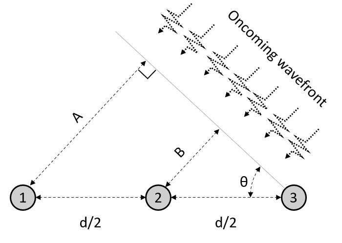A Simple 3-mic setup with a sample oncoming wave

As a recap, let us visualise how each of the signals are arriving at the three mics, and the aggregate recordings of the 3 mics (again, the mics only record the aggregate signals, and not the individual frequency components)

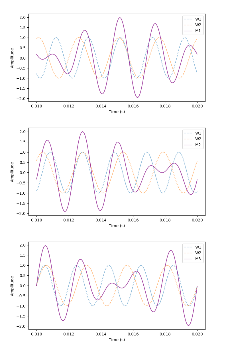Multiple Monotone waves from different angles: Mic Recordings

The aggregate array response along with the individual mic recordings are also plot for reference:

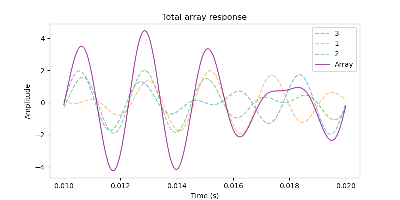Multiple Monotone waves from different angles: Array recording

Since this methodology did not work in the time domain, we have to extract the two waves out from the composite waves in each microphone. As an experimental setup, we only have the individual mic recordings available with us. From this, we have to extract the individual frequency components. This takes this problem to the frequency domain. Even though the beamforming process fundamentally remains the same, the specifics change a little. We will now:

_

1. Take the Fourier Transform of the signal recorded in each microphone. Separate out the each of the individual signals (specifically, the amplitude and phase [1]).
2. “Steer” (iterate) over various angles (and hence, various time delays) in the frequency domain. For each iterating angle, calculate and recover the time delay on each of these frequency components individually, again continuing in the frequency domain itself.
3. Then sum this signal across the three mics to obrain the aggregate array recording and response. For each angle, as many responses (called beamformer output) are obtained as many individual frequency components are present. This is classic Delay-and-Sum Beamforming.
4. The angle for which the beamformer output is maximum is the angle of incidence for that particular frequency component as per this beamformer model.

… I know this sounds a little too complex, but this is literally what we did in the time domain, but now we have to follow this in the frequency domain. We will follow the above methodology step by step for a better understanding.

_

1. Fourier Transform for each mic recording [2]

Firstly, we will take the Fourier Transform of the signals in each of the mics to extract the information of individual frequency components. Following the procedure as explained in the Fourier Transform post, we obtain the below:

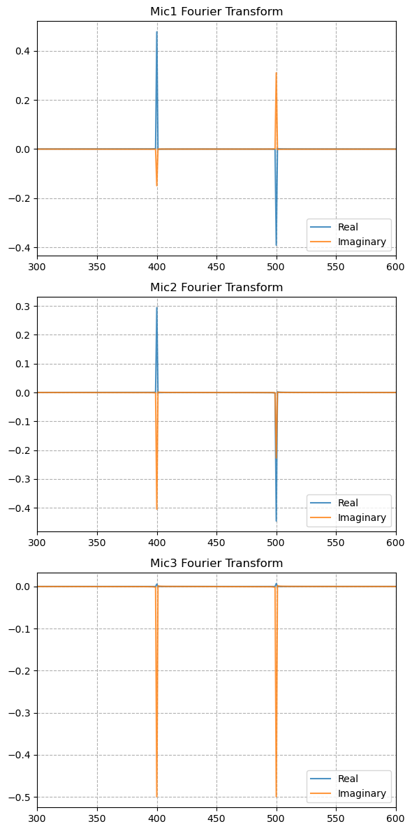Fourier Transforms of signals in each mic

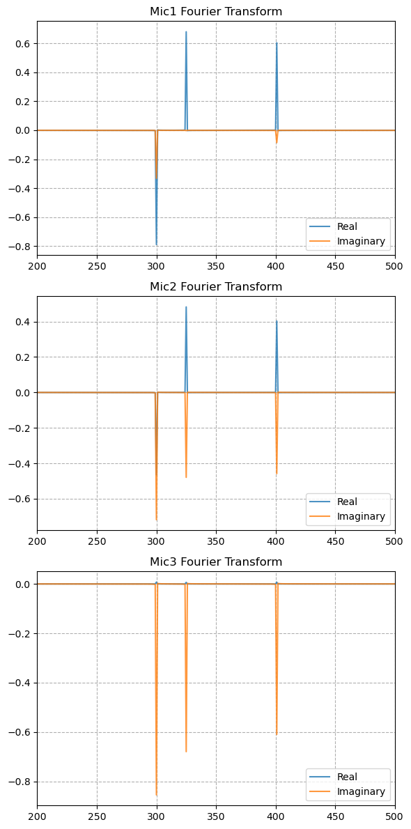
You can notice that the two signals (400Hz and 500Hz) now have been separated! Also, as explained in the post about investigations into the Fourier Transforms, the Real and Imaginary values of the FT combine to give the amplitude and phase information of that frequency signal in the composite wave!

Both the real and imaginary components together convey information for both the AMPLITUDE and the PHASE of the wave at $t=0$

Now that the signals are separated in each mic, we will steer through various angles scanning for these same individual frequencies.

2. Steering: Frequency domain

In this section, we will go through the “steering” process in the frequency domain.

If you recall, in the time domain, we had recovered the time delay for a given microphone by advancing the signal by the computed time delay for that iterable angle $\theta_0$. Mathematically, if the actual signal in a given mic $i$ is $s_i(t) = s(t - td_{i_actual})$, then for the given iterable angle $\theta_0$, the time-advanced signal for the mic:

\[s_{ia}(t) = s_i(t + td_{i}(\theta_0))\]

where $td_{i}(\theta)$ is the time delay calculated for $\theta_0$. For example, in this scenario, for mic 1:

\[s_{1a}(t) = s_1(t + td_{1}(\theta_0)) = s(t - td_{1actual} + td_{1}(\theta_0))\]

where, for a signal of speed $c_0$

\[td_1(\theta_0) = \frac{d\mathbf{sin}\theta_0}{c_0}\]

And as we had discussed earlier, constructive interference happens when the time advance exactly equals the time delay so that the signals in each of the mics are all in-phase to output a maximum array response. Now, we just have to replicate this concept in the frequency domain. For this, we need to understand how the time delay or advancement looks like in the frequency domain.

This has already been discussed here, and the concept is called Fourier Shift Theorem.

This concept states that, for any time delay of a signal in the temporal domain, it translates to a multiplicative phase factor in the frequency domain. If the Fourier Transform of a signal $x(t)$ is

\[FT(x(t)) = X(f) = \int_{-\infty}^{\infty} x(t)\mathbf{e}^{-j2\pi ft}dt\]

Then

\[FT(x \left( t - t_m \right) ) = \mathbf{e}^{-j2\pi ft_m} X(f)\]

In our case, the Fourier Transforms have already been computed for the signals in each of the three mics. Let us call them $X_i(f)$, and in this example $f$ has the discrete values of 400Hz and 500Hz, since the FT is zero for all other values.

Now, we will calculate the time delay in all the three mics for a given iterable angle $\theta_0$. As calculated earlier,

\[td_1(\theta_0) = \frac{d\mathbf{sin}\theta_0}{c_0}, \qquad td_2(\theta_0) = \frac{d\mathbf{sin}\theta_0}{2c_0}, \qquad td_3 = 0\]

The corresponding signals after processing (i.e., advancing in time to recover the time delay) in each of the mics are $s_i(t + td_{i}(\theta_0))$ for a given mic $i$.

In the frequency domain, applying the Fourier Shift theorem:

\[FT \left( s_i(t + td_{i}(\theta_0)) \right) = \mathbf{e}^{-j2\pi f \left( -td_i(\theta_0) \right) } X_i(f) = \mathbf{e}^{j2\pi f \left( td_i(\theta_0) \right) } X_i(f)\]

_

Notice that the exponent does not have a negative power, since we are not delaying but advancing to recover for the time delay.

This exponential term is actually called the Steering Vector. It is called a vector because it is pointing to the different angles when iterating, to identify the noise sources. [3]

\[SV_i(f, \theta_0) = \mathbf{e}^{j2\pi f \left( td_i(\theta_0) \right) }\]

As can be observed, every mic $i$ has a steering vector at a given iterable angle $\theta_0$ for all the frequency components incident on it. Hence, the time advanced signals in frequency domain for any given mic $i$ is:

\[SV_i(f, \theta_0) X_i(f)\]

For proper understanding, we will now analyse per individual frequency component / signal. For the 400Hz component, the steering vectors are:

\[SV_1(\theta_0) = \mathbf{e}^{j2\pi \ * \ 400 \ * \ \left( td_i(\theta_0) \right) } = \mathbf{exp} \left( j2\pi \ * \ 400 \ * \ \left( \frac{d\mathbf{sin}\theta_0}{c_0} \right) \right)\]

Similarly,

\[SV_2(\theta_0) = \mathbf{exp} \left( j2\pi \ * \ 400 \ * \ \left( \frac{d\mathbf{sin}\theta_0}{2c_0} \right) \right), \qquad SV_3(\theta_0) = \mathbf{exp} \left( j2\pi \ * \ 400 \ * \ \left( 0 \right) \right) = 1\]

The corresponding time-advanced signals in frequency domain $SV_i(f, \theta_0) X_i(f)$ are:

\[\mathbf{exp} \left( j2\pi \ * \ 400 \ * \ \left( \frac{d\mathbf{sin}\theta_0}{c_0} \right) \right)X_1(400), \qquad \mathbf{exp} \left( j2\pi \ * \ 400 \ * \ \left( \frac{d\mathbf{sin}\theta_0}{2c_0} \right) \right)X_2(400), \qquad X_3(400)\]

3. Summation of each mic signal

The aggregated signal recording of the array is, as is the case in temporal domain, a summation of the time-advanced signals in each of the 3 mics.

\[\sum_{i=1}^{3}SV_i(400, \theta_0) X_i(400) = \mathbf{exp} \left( j2\pi \ * \ 400 \ * \ \left( \frac{d\mathbf{sin}\theta_0}{c_0} \right) \right)X_1(400) + \mathbf{exp} \left( j2\pi \ * \ 400 \ * \ \left( \frac{d\mathbf{sin}\theta_0}{2c_0} \right) \right)X_2(400) + X_3(400)\]

The Beamformer output (let us call it $BF$) is but the square of this summation. Thus, for the 400Hz signal, at any given iterable angle $\theta_0$,

\[BF(400, \theta_0) = \left( \sum_{i=1}^{3}SV_i(400, \theta_0) X_i(400) \right)^2\]

This same process is to be repeated for the 500Hz component, or any other if present. Thus, formally:

\[BF(f, \theta_0) = \left( \sum_{i=1}^{3}SV_i(f, \theta_0) X_i(f) \right)^2\]

4. Iterate over each angle $\theta_0$

The next step is to iterate over $\theta_0$. In the above equation, the Beamformer output is computed across various values of $\theta_0$, and the $theta_0$ at which the output is maximum is the angle at which the particular frequency component signal is incident on the array setup.

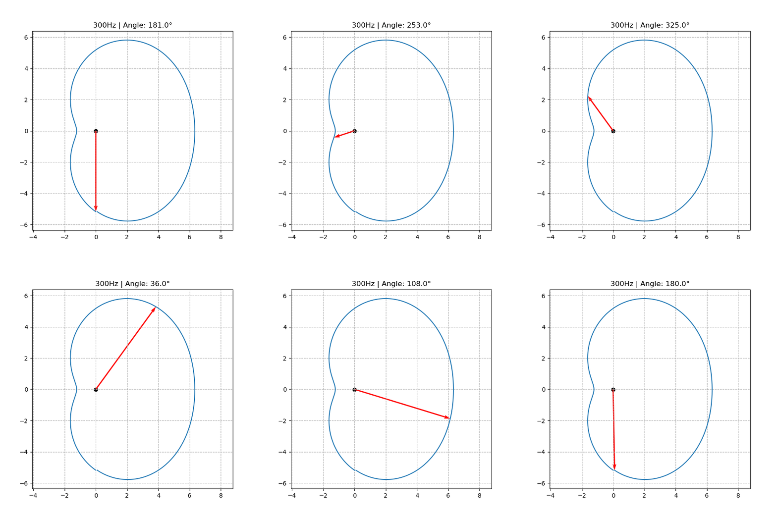
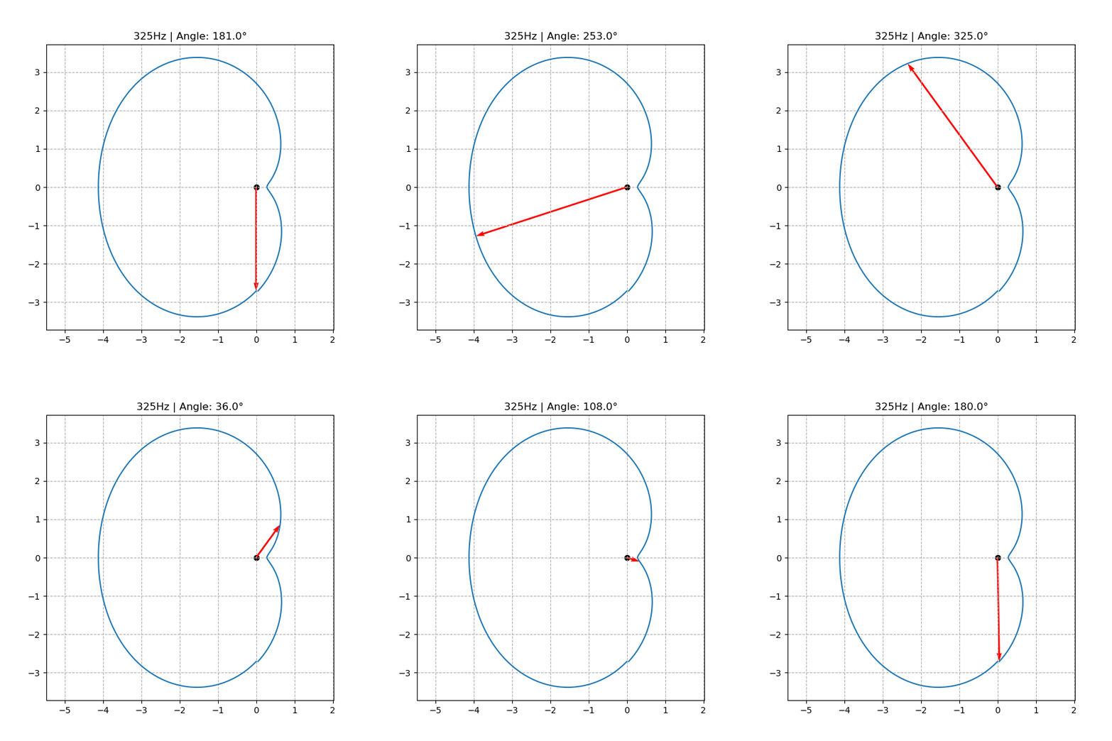
Now, let us visually understand this procedure. For this, I tweaked a certain trick. I have plot in a cartesian grid, a “circle”, with variable radius. At each angle, the radius is equal to the Beamformer output. This way, we can see from where the signal is coming from!

Take the case of the 400Hz signal.

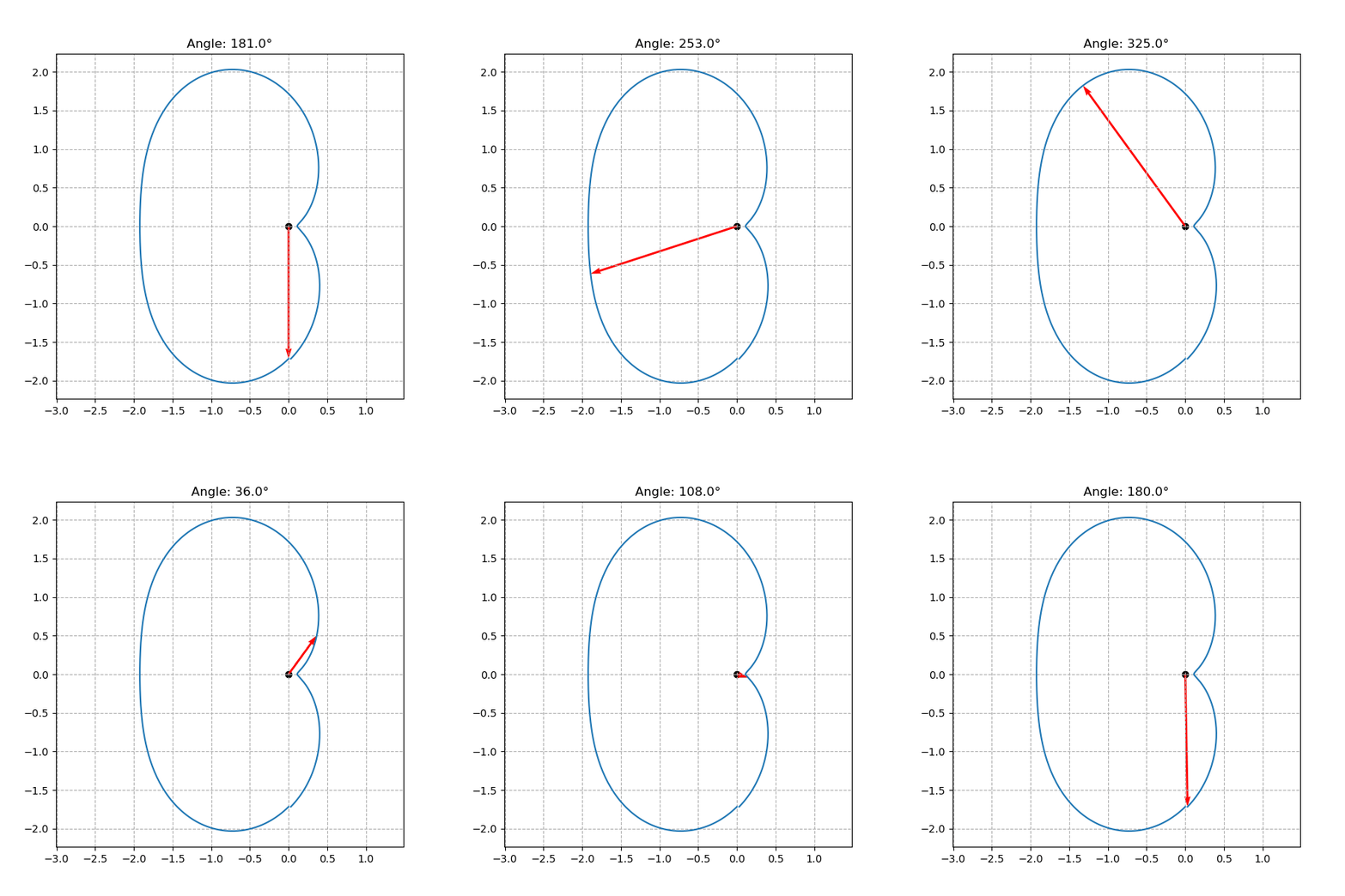Beamformer output for 400Hz component

You can notice that the value is maximum at around 325°, as is the actual case! The above visualisation actually helps us understand the term “beam” in beamforming. The array setup actually projects a “beam” to the signal source region, thus effectively identifying it. Now we will plot the response vs angles for 400Hz component

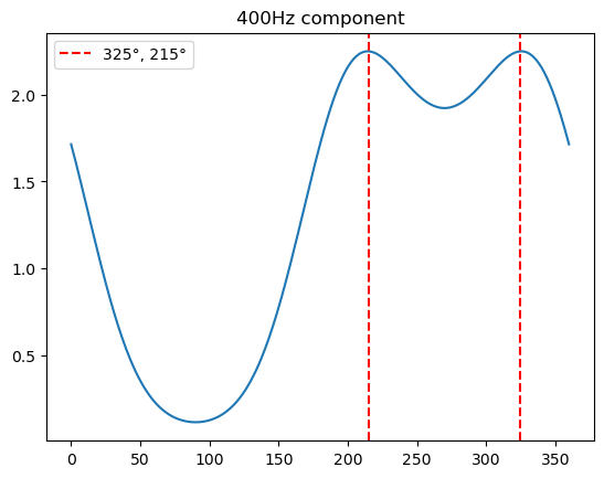Beamformer output vs angles for 400Hz component

And this time, it worked! Unlike the temporal beamformer. Keep in mind that the prediction of 215° also as a possible angle is because of the symmetry of the array setup to the two angles of incidences, as discussed in previous post as well. This is a limitation of using a 1D array setup. Also check the 500Hz component:

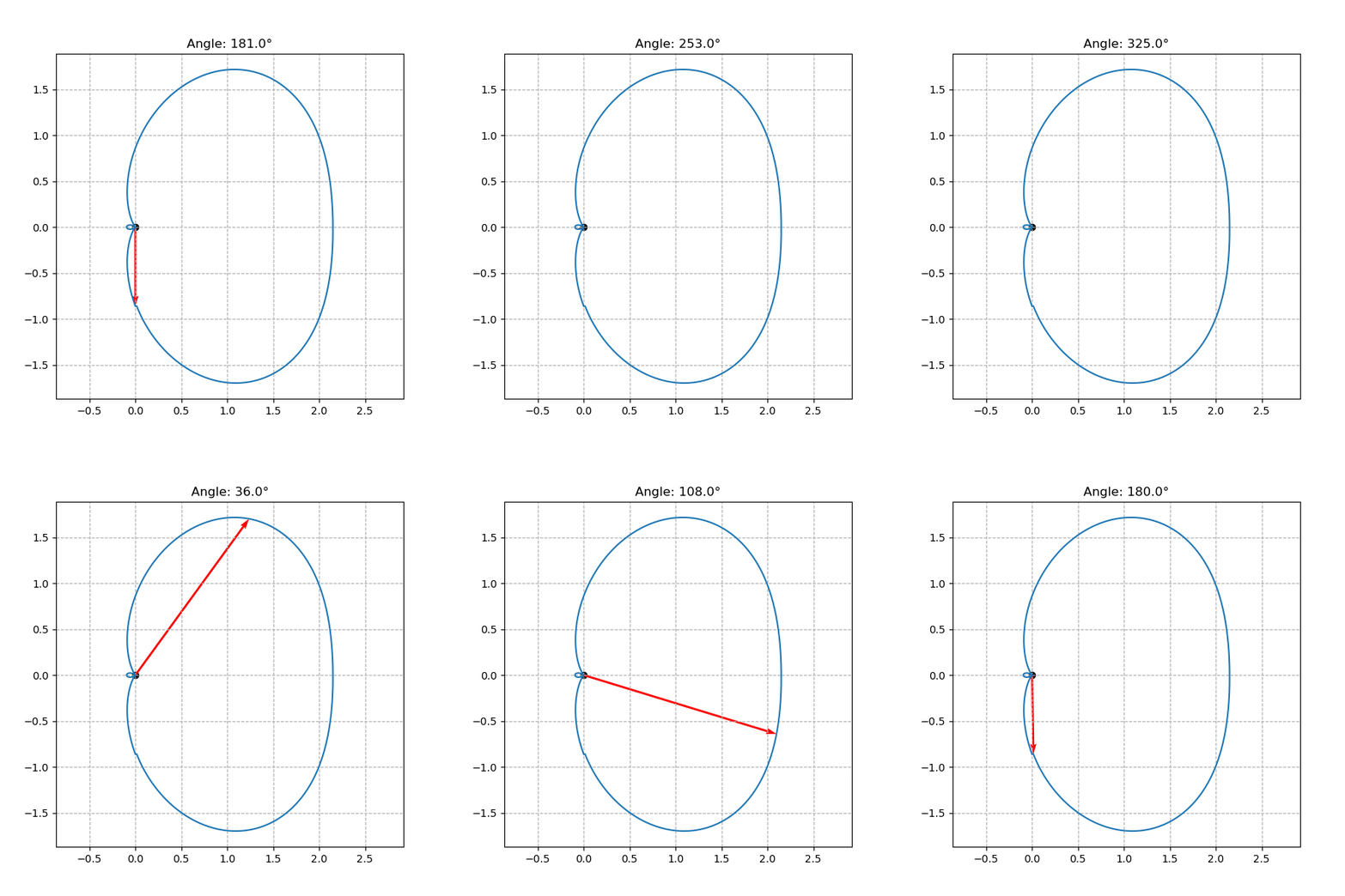Beamformer output for 500Hz component

And the response vs angles:

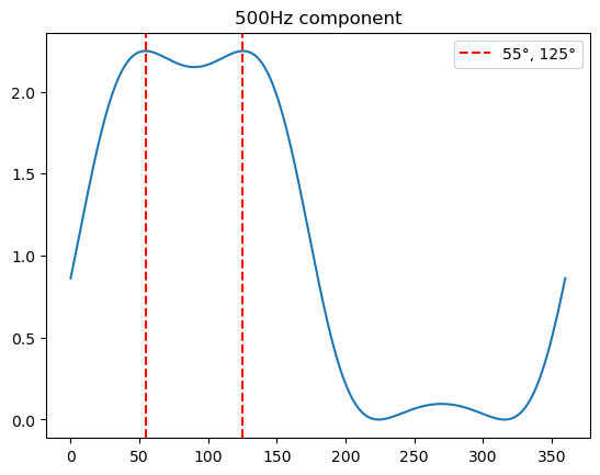Beamformer output vs angles for 500Hz component

The beamformer setup is able to predict accurately for the 500Hz component as well!

Now, we will explore even further examples to understand this setup better. Specifically, to understand the response value of the beamformer array setup.

Example 2: Understanding the Beamformer output value

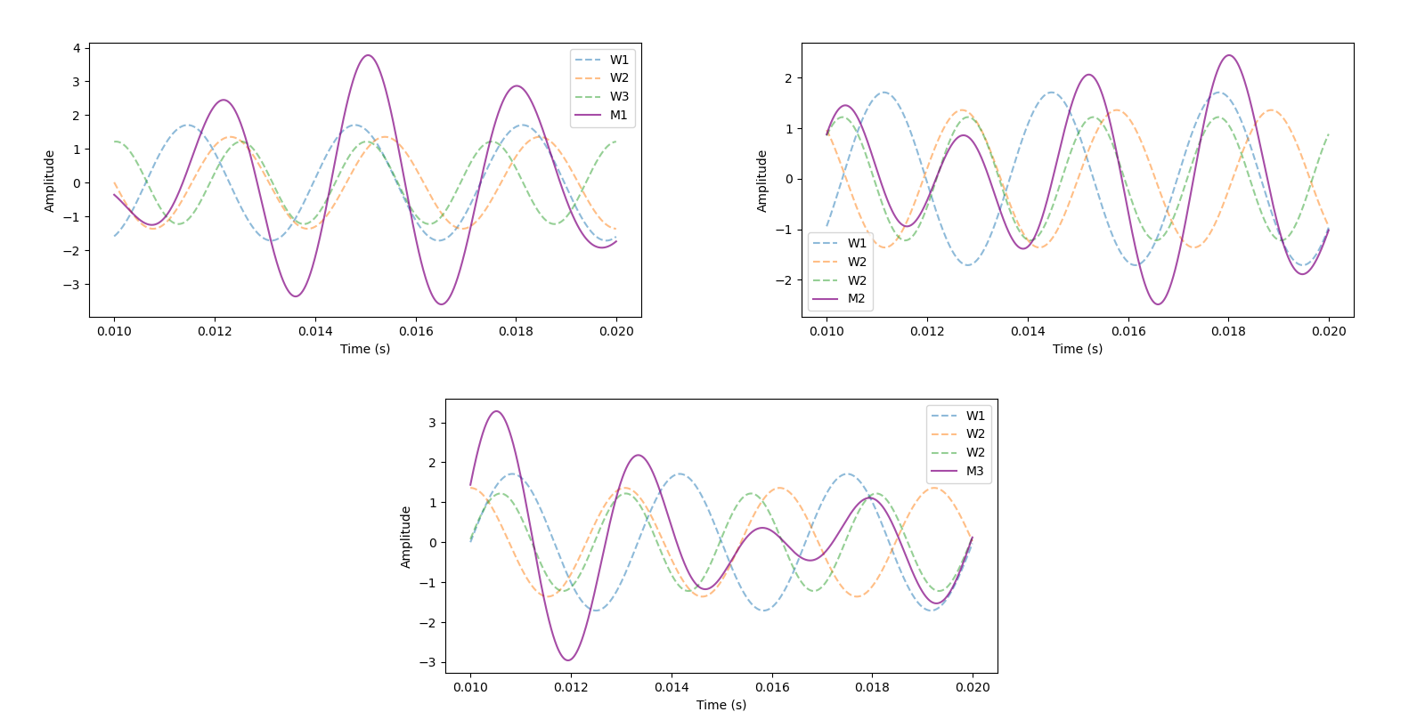
We will firstly take another example, but this time consisting of different frequencies of varying amplitudes. Consider these 3 signals:

1. 300Hz, 1.71 Amplitude, at 46°
2. 325Hz, 1.36 Amplitude, at 300°
3. 401Hz, 1.22 Amplitude, at 320°

The aggregated signals received in each mic looks like:

Example 2: Signals received at each mic

Now we will proceeed step by step. Firstly, taking the Fourier Transforms of the aggregated signal recordings at each mic:

Example 2: Fourier Transforms of signals in each mic

Now, we will Delay and Sum Beamform. The “Beamforming plot” is shown for each frequency component below:

Beamformer output for 300Hz component

Beamformer output for 325Hz component

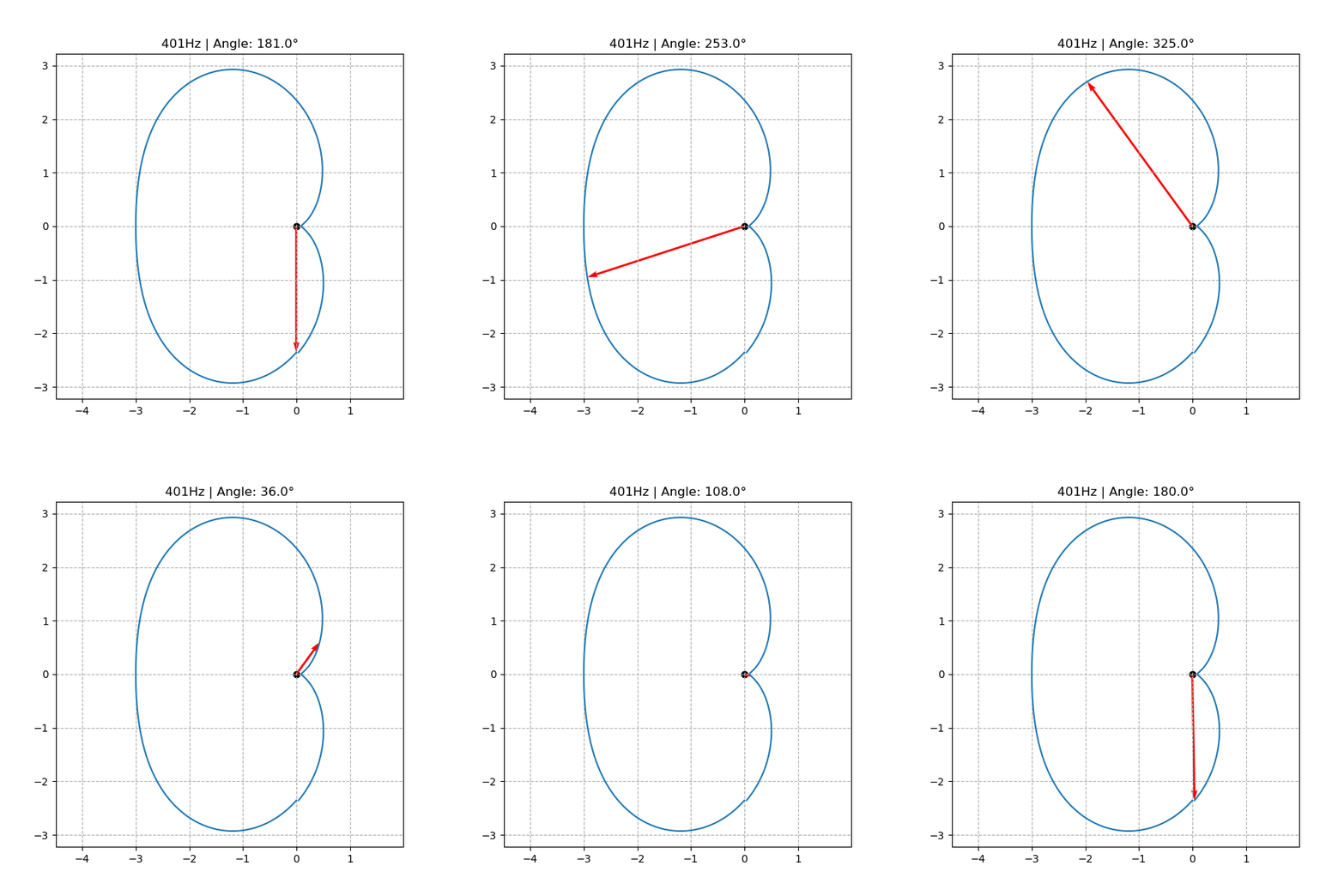Beamformer output for 401Hz component

The corresponding responses for each angle for all the individual frequency components is plot below:

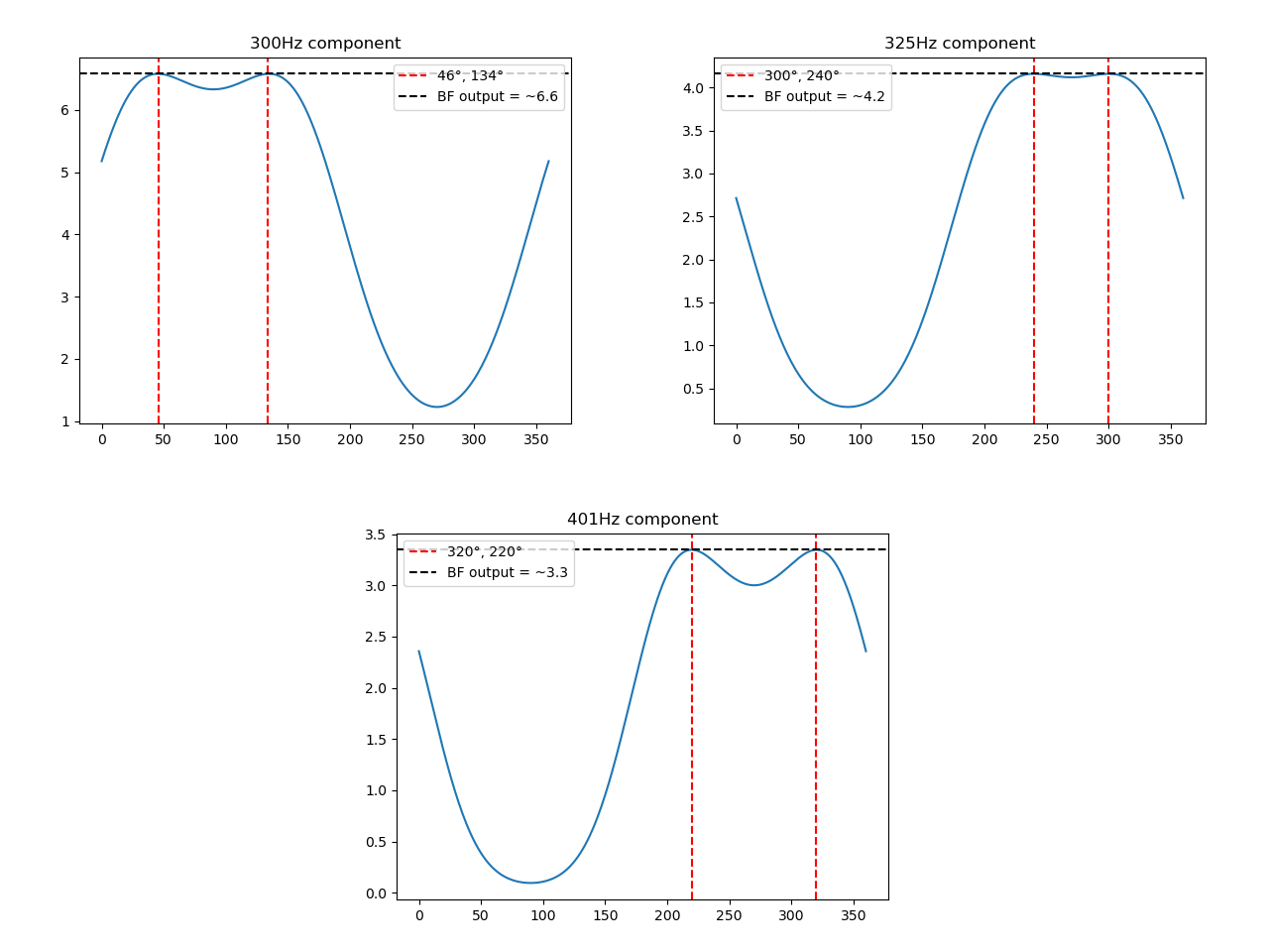Beamformer output vs angles for each individual component

This algorithm has been succesfull at predicting the direction of each of the incident signals! Yes, the symmetry of a 1D array setup does pose problems, but that can be very easily overcome.

One more thing to notice is that, the Beamformer is also able to capture the amplitude in some way. In our signal setup, 300Hz had the highest amplitude, followed by 325Hz and 401Hz respectively. This same sequence is followed in the Beamformer responses as well. This suggest some kind of relation between the two.

Technically, what the Beamformer does is align all the signals across various microphones completely in-phase such that, when they are summed they constructively add up.

\[BF(f, \theta_0) = \left( \sum_{i=1}^{3}SV_i(f, \theta_0) X_i(f) \right)^2\]

When the value of $\theta_0$ is equal to the actual angle of incidence of the particular frequency component, that is when the signals from each mic constructively add up.

_

And, from my investigations into the Fourier Transform, it is found that the amplitude of the Fourier Transform is exactly HALF of that of the signal amplitude in the time domain. Say the amplitude for a given frequency component is $A(f)$, and if $N$ is the number of mics, then the output is simply the base signal multiplied by a factor of number of mics. [4]

\[BF(f, \theta_0 = \theta) = \left( \frac{NA}{2} \right)^2\]

In this case, the Beamformer response for each of the signals are:

\[BF(300) = (0.5*3*1.71)^2 = 6.579\] \[BF(325) = (0.5*3*1.36)^2 = 4.16\] \[BF(401) = (0.5*3*1.22)^2 = 3.3489\]

_

Which is exactly what the Beamformer also calculated! Thus, the DAS Beamformer not only captures the direction of the individual frequency components incident on the setup [5], but also their respective amplitudes.

Example 3: Two signals from different directions, but same frequency

This is one final example we shall experiment on. In this, we shall see if the Beamformer array is able to distinguish between two signals of the same frequency, but from different directions.

As an example, we shall consider two 300Hz signals:

1. 1.34 Amplitude, 46°
2. 1.02 Amplitude, 300°

The Fourier Transforms are plot here:

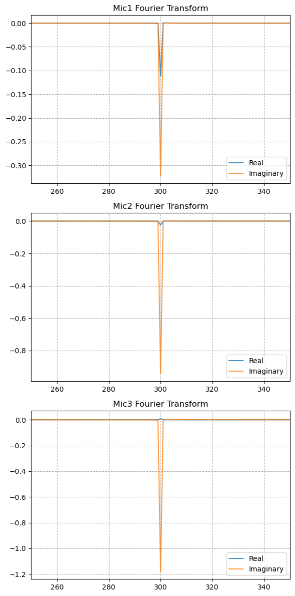Example 3: Fourier Transforms of signals in each mic

Here itself we can notice something.. ofcourse, the Fourier Transform has filtered out the 300Hz signal. But there seems to be no distinction between the two different 300Hz signals, they seemed to be clubbed together to output the Real and Imaginary Fourier Transform values. Anyway, proceeding to the next step: DAS Beamforming

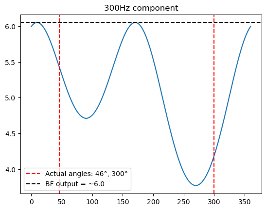Beamformer output vs angles for 300Hz component

The Beamformer seems to have completely collapsed, here! Not only is the directions predicted very wrong, but even the amplitude of the BF response is way off the mark.

This is one major limitation of this array setup. The calculations itself are not wrong, but having just 3 microphones that too in a 1D array, is not optimal. Not only does the symmetry cause problems, but also this setup is not able to distinguish between two different signals from different directions, but having the same frequency. This is because this Beamformer array assumes one direction for one particular frequency signal ; for one set of Real and Imaginary values of the Fourier Transform. If the signals, even if from different directions, are having the same frequency, the Fourier Transform does not distinguish between the two. The FT is a tool to extract individul frequency elements, but not spatially distinguish them.

Anyway, this limitation is overcome by adding plenty more microphones, and in a 2D setup such that the signals are incident perpendicular to the array plane.

For now, I shall stop the investigation here. In the next post, I shall explain in detail a real-world engineering use-case Beamformer array.

Footnotes

_

[1] The angle of incidence directly influences the phase of the signals incident on the array setup.

_

[2] For an easy approach, a software tool is used for Fourier Transformation. Nevertheless, the procedure and fundamentals are the same as in the posts on Fourier Transform. (1) (2)

_

[3] The definition of the Steering Vector for this scenario in my python code is:

def steering_vect(d, theta, f):
    c0 = 340
    td2 = 0.5*d*np.sin(theta*np.pi/180)/c0
    td1 = d*np.sin(theta*np.pi/180)/c0
    sv2 = np.exp(-2*np.pi*f*1j*td2)
    sv1 = np.exp(-2*np.pi*f*1j*td1)
    return np.array([sv1, sv2, 1])

Which is basically,

\[SV_i(f, \theta_0) = \mathbf{e}^{-j2\pi f \left( td_i(\theta_0) \right) }\]

Notice that unlike in my process definition here, I do use the negative exponent. It is because, the summation part of this algorithm:

\[\sum_{i=1}^{3}SV_i(f, \theta_0) X_i(f)\]

is nothing but a vector dot product

\[SV_i(f, \theta_0) \cdot X_i(f)\]

where for a particular frequency and iterable angle $\theta_0$, both the quantities are a row/column vector of shape (number_of_mics, 1)

In python, this is written as:

thetas = np.linspace(0, 360, 361)
for f in [400, 500]:
    for theta0 in thetas:
        a = steering_vect(d = 0.3, theta = theta0, f = f) # d = 0.3, space between mics 1 and 3
        bf_val = np.abs(np.vdot(a, FT[f]))**2

And in the very definition of np.vdot (refer python documentation here), “if a is complex the complex conjugate is taken before calculation of the dot product”. The complex conjugate of the steering vector as per the code definition is:

\[\bar{SV_i}(f, \theta_0) = \mathbf{e}^{j2\pi f \left( td_i(\theta_0) \right) }\]

Which matches the definition in my process explanation.

_

[4] A simple multiplication by number of mics is not always true. It is true in this scenario simply because of the simplicity of the setup. Nevertheless, the BF response is proportional to or a factor of the number of mics in the array setup.

_

[5] This is an important part to understand. Even the amplitudes of signals captured by the array setup is not the actual source noise amplitude, but the amplitude sensed by the array setup. Technically, the signals from the noise source will dampen/decay by the time it reaches the array setup, thus leading to under-prediction of the amplitudes. But that is OK, since it happens to every single signal, and as a relative, comparative analysis, it works.

[6] The codes for images and animations generated by self, and even further, are consolidated here.