Investigations into the Fourier Transform - 1

In the earlier post, I’d elaborated on the visualisation of the Fourier Transform, partly from the beautiful video of 3B1B and partly my own explorations. I did not stop exploring my understanding, but investigated further to understand some questions which, one by one, naturally arose. Some of the crucial aspects I shall be jotting down here.

1. The Half-Value

As had been observed earlier, the centroid of the “wrapped wave” tends to shift AWAY from the origin when the “wrapping frequency” matches the wave frequency itself. Take the case of a pure 5Hz sine wave here:

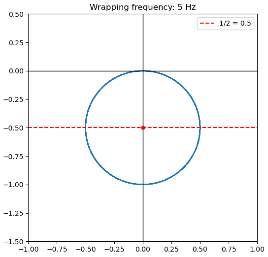Wrapping of 5Hz wave at 5Hz

Notice how the coordinate of the centroid is HALF of the amplitude of the wave. Naturally, I found a pattern when handling different signals, both tonal and composite. For example, for a composite wave having 2 pure sine waves, of frequencies and amplitudes (10Hz, 6Hz) and (1.3, 0.7) respectively, the wave in the frequency domain at the specific “wrapping frequencies” looked like this:

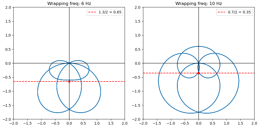Wrapping of composite wave (6Hz + 10Hz)

Notice again, the coordinate centroid for each case is HALF of the amplitude of each of the specific frequencies IN THAT WAVE. Now, that seems fascinating. Let us investigate further. For now, I will ignore the x- and y-coordinate distinction of the centroid in the complex plane and focus only on the y-coordinate. Specifically, the negative y coordinate. Again, more on this later.

Firstly, we will visualise the wrapping of the wave in the complex plane. Say, take the case of the 5Hz pure sine wave.

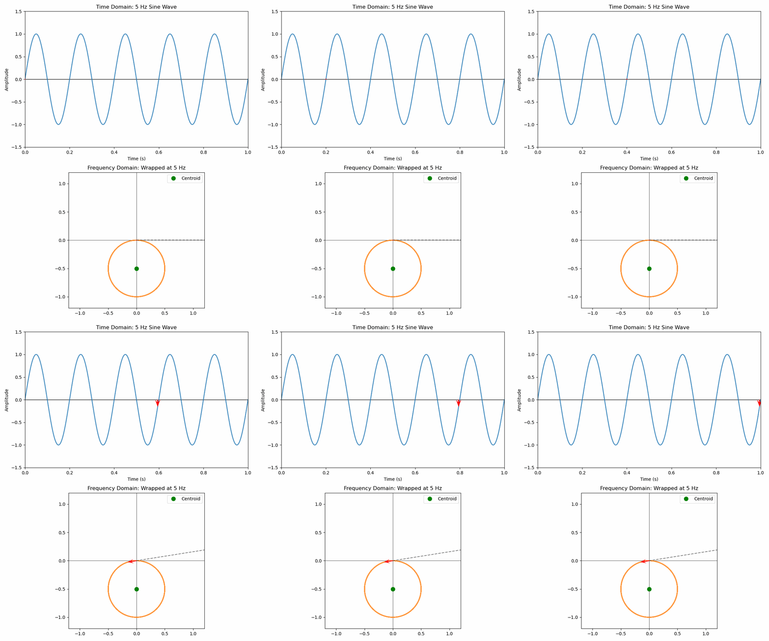Wrapping of 5Hz wave at 5Hz

Since the “wrapping frequency” is 5Hz, it means that one “wrapping” revolution around the complex plane is completed in (1/5) seconds. In other words, one time period - or one oscillation - of the wave is covered in one rotation, since the time period of the wave is also (1/5) seconds.

Let us observe the first half rotation in the complex plane. As expected, it is tracing the half-wave (positive) amplitude oscillation and forming a perfect circle as a consequence. Since the wrapping is clockwise from the +x axis (as a convention), the circle is formed in the bottom half of the plane.

Now, what happens in the 2nd half-wave oscillation? Since the wave is exactly the same as the first half but with a negative amplitude, the “wrapping” simply retraces the existing circle, instead of creating a circle in the top half. This leads to the centroid (y) coordinate to be exactly half of the maximum amplitude of the wave, which is, in this scenario, lying on the (-)y axis, at 90 degrees from the wave.

Similarly, if you take the Fourier Transform of any composite wave, the centroid coordinate (which, as in the previous post, is essentially the Fourier Transform), will be exactly half of the amplitude of the particular frequency wave in the composite signal.

But this is only a geometric intuition of the half-value of the Fourier Transform. How do you understand it mathematically, in the complex plane?

Earlier, we had established the Euler’s Formula for complex numbers:

\[\mathrm{e}^{ix} = \mathrm{cos}x + i\mathrm{sin}x\]

From this, it can be derived that:

\[\mathrm{cos}x = \frac{\mathrm{e}^{ix} + \mathrm{e}^{-ix}}{2}\]

and,

\[\mathrm{sin}x = \frac{\mathrm{e}^{ix} - \mathrm{e}^{-ix}}{2i}\]

Since the above example is a sine wave, we will look at the second equation. Let us also consider it having an amplitude $A$, say. In that case, for the frequency $x$ of the sine wave, the amplitude $A$ in the frequency domain - or, the “wrapping” plane - when wrapped at a frequency $x$ is split halfway between the positive and negative of the frequency $x$ as per Euler’s formula.

\[A\mathrm{sin}x = A\frac{\mathrm{e}^{ix} - \mathrm{e}^{-ix}}{2i} = \frac{A}{2i}\mathrm{e}^{ix} - \frac{A}{2i}\mathrm{e}^{-ix}\]

Multipling numerator and denominator of RHS by $i = \sqrt{-1}$,

\[A\mathrm{sin}x = -\frac{A}{2}i\mathrm{e}^{ix} + \frac{A}{2}i\mathrm{e}^{-ix}\]

Notice that the amplitude $A$ is split between two frequencies (of “wrapping”) here. $-Ai/2$ for the $+x$ frequency, and $Ai/2$ for the $-x$ frequency. This “splitting” of amplitude across +/- frequencies is called Hermitian Symmetry. But what exactly is a “negative” frequency of wrapping? It is simply wrapping the wave counter-clockwise around the complex plane from the +x axis. For example, the same 5Hz case when wrapped at (-)5Hz frequency, we obtain this:

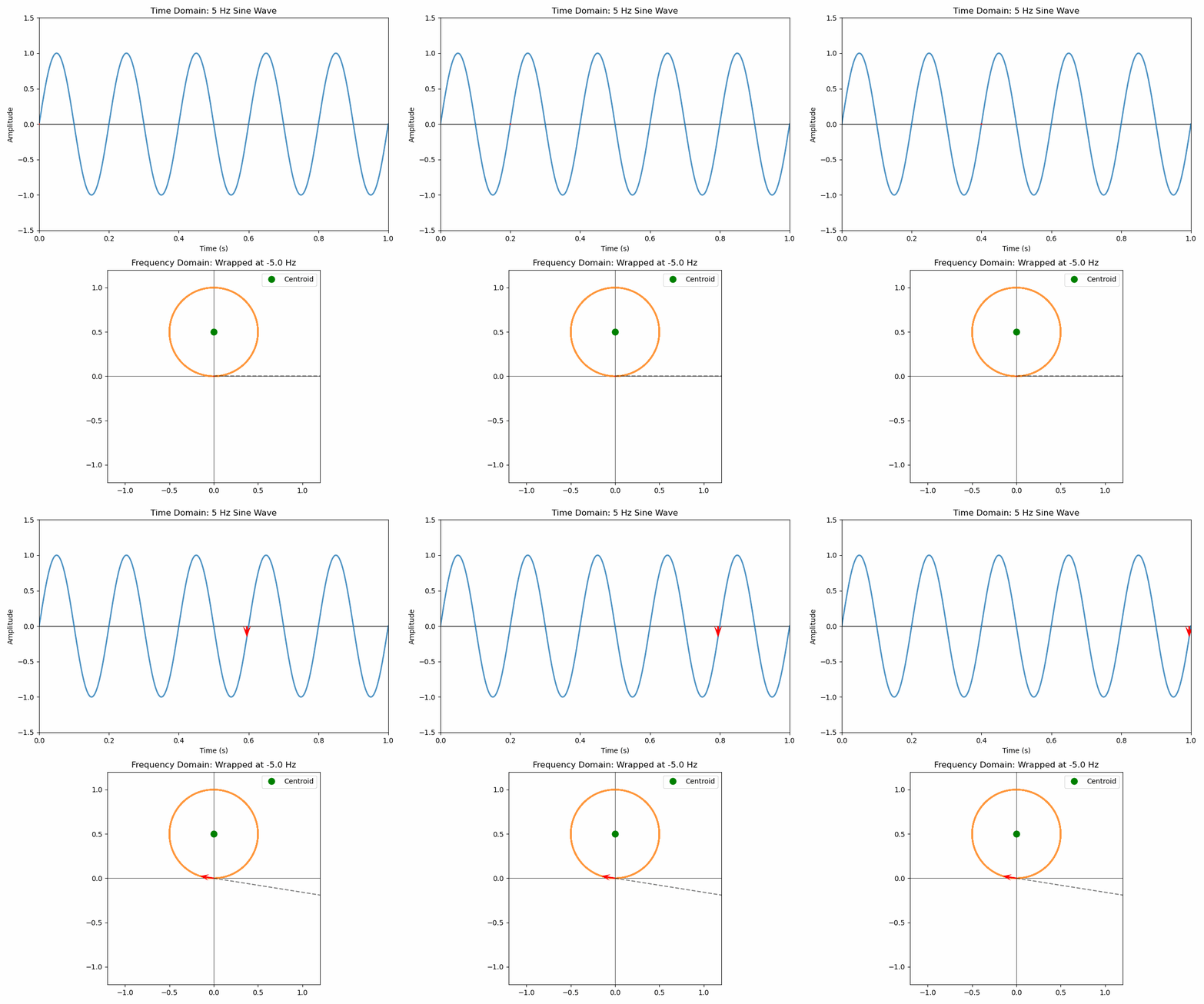Wrapping of 5Hz wave at -5Hz

See how the centroid is now located at $+Ai/2$!

Now, if we plot the y-coordinate of the centroid against frequency, we can notice the + and - peaks of $A/2$ at the negative and positive frequencies respectively:

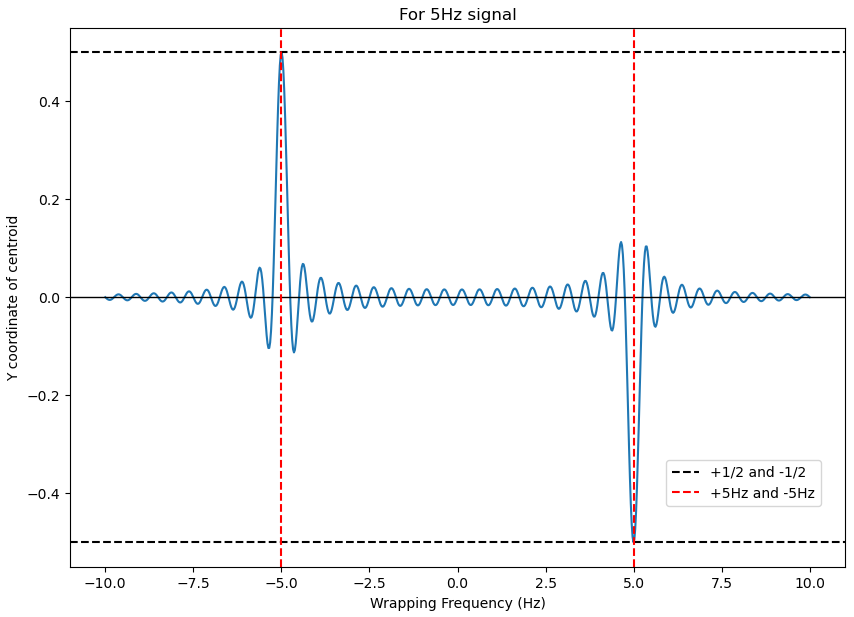Y coordinate of the centroid of 5hz sine wave wrapped at various frequencies

So, naturally, we can ask:

• What is this “negative frequency” of wrapping?
• What happens when you take the case of the cosine wave? Or a phase-shifted sinusoidal wave? Or a combination of several such phase-shifted waves?
• Why did I only plot the y coordinate? What are the x and y coordinates?

By now, one must - mostly - have gotten an idea.

2. The Axes in the Complex Plane

Before investigating those questions, first we will now shift our “wrapping’ examples from the sine waves to the cosine waves. How does the Fourier Transformation of the cosine waves look like?

The 0° starts from the +x axis, and the cosine wave starts from a peak amplitude value, say 1 here. So, for a 5Hz wave, wrapped at 5Hz in the complex plane, the figure would look something like this:

_

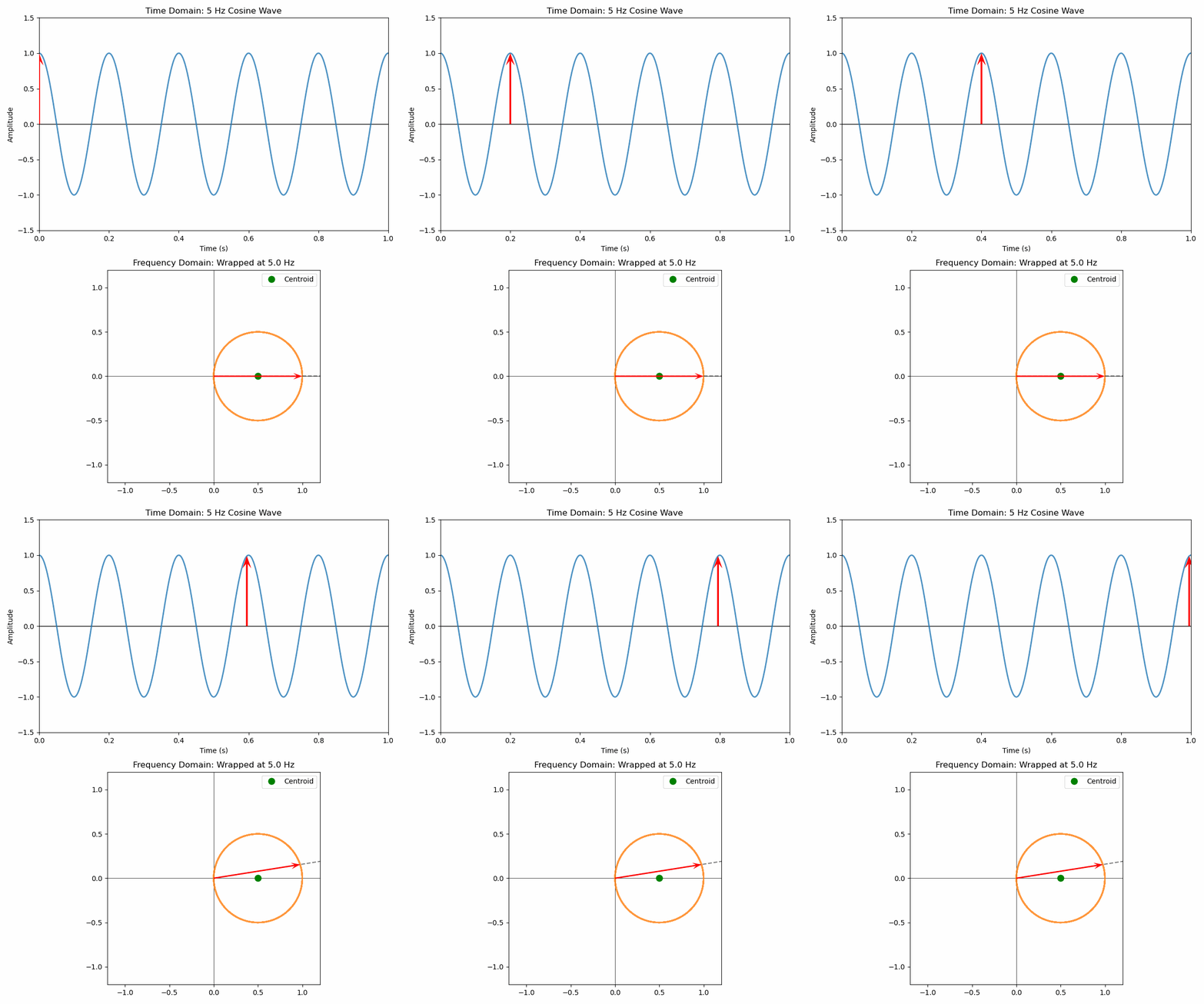Wrapping of 5Hz cosine wave at 5Hz

The centroid is now lying on the real axis of the complex plane. So, what if I take a slightly phase-shifted sine wave? Say the phase shift is by 30° of the wave oscillation (one wave oscillation has 360°). In that case:

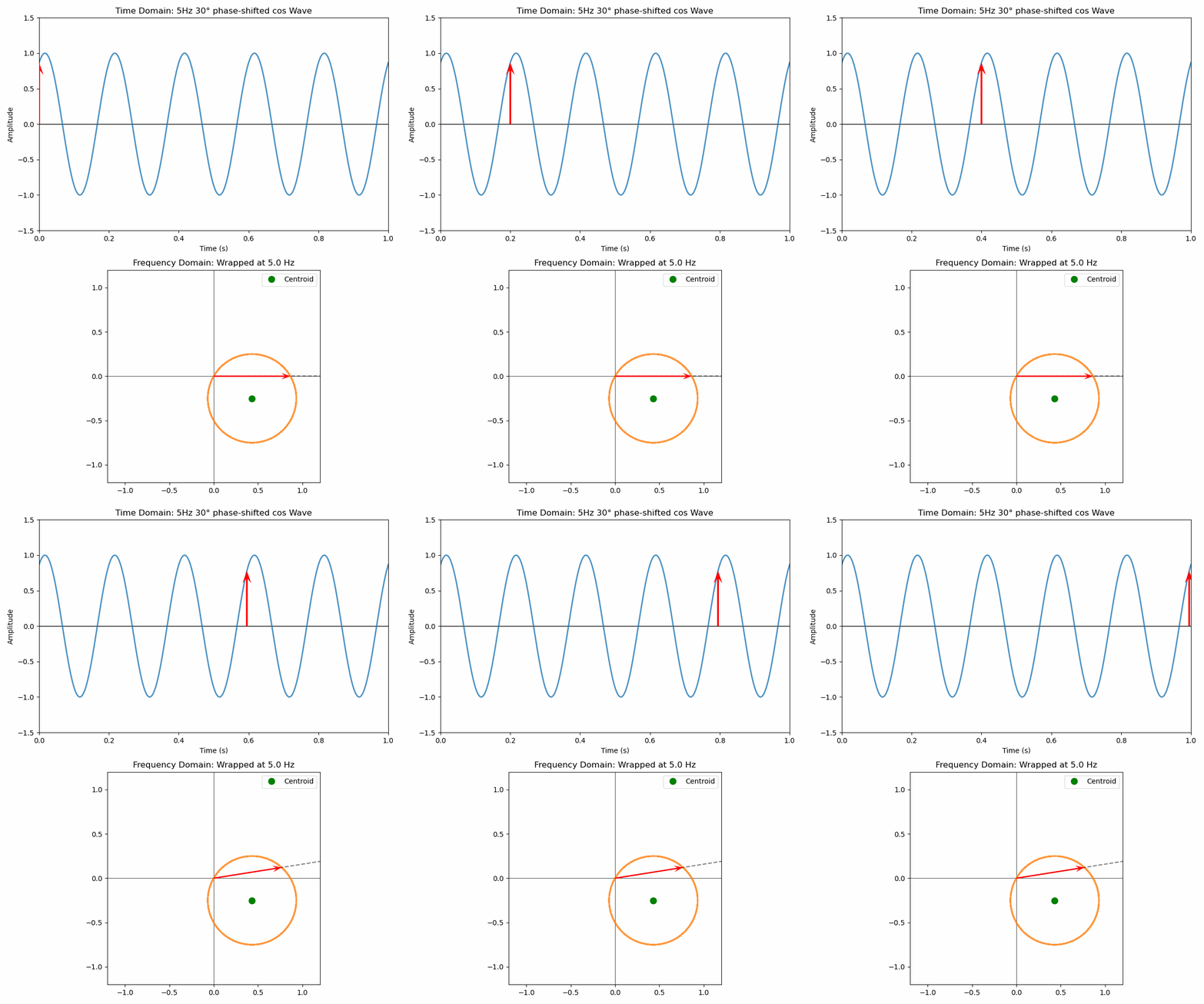Wrapping of 5Hz 30° phase-shifted cosine wave at 5Hz

Notice that it seems simply shifted (or better yet, rotated (AGAIN!)) the circle by 30° clockwise from the +x axis. Let us test this hypothesis. If true, the sine of this phase-shifted angle in the frequency domain (which basically would be the y-coordinate of the centroid) will be $\mathrm{sin}30^{\circ}$

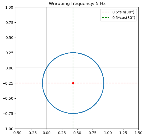5Hz 30° phase-shifted cosine wave wrapped at 5Hz: Coordinates of centroid

By now, it should be mostly clear how this “circle” moves with respect to the phase shift of the pure sinusoidal wave. It can be visualised below:

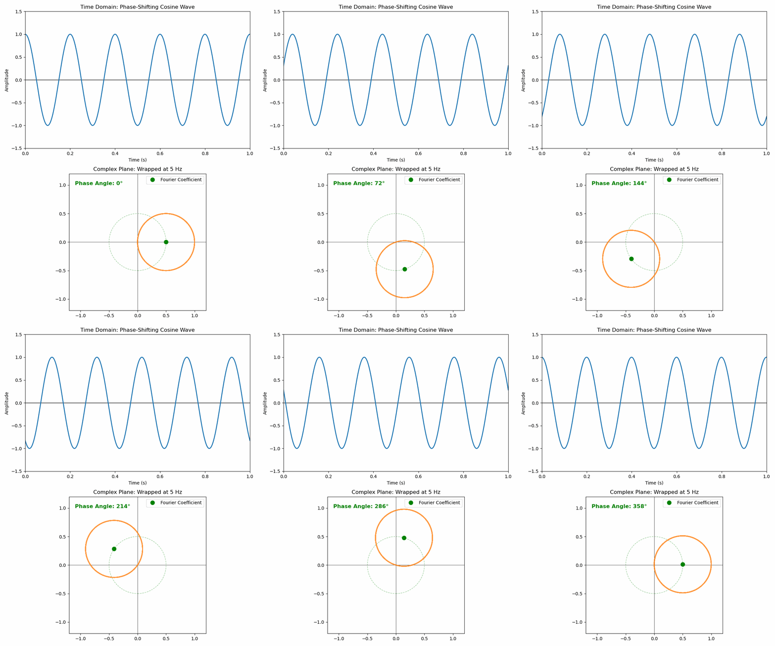Phase Shifting a 5Hz sinusoidal wave

_

Hence, a signal wrapped in the complex plane, rotates clockwise when the same signal is DELAYED in time. The rotation changes the value of the Fourier Transform, with the cosine of the phase shift representing the value in the REAL axis, and the sine in the IMAGINARY axis. In the “Fourier World”, a cosine is the fundamental wave, which rotates clockwise when you delay the wave in time. This is fundamentally called the Fourier Shift Theorem [3]

So, for ANY particular wave, the Fourier Transform at a particular frequency (i.e., when “wrapped” at a particular frequency) is a COMPLEX number. Both the real and imaginary components together convey information for both the AMPLITUDE and the PHASE of the wave at $t=0$.

Hence, at whatever be the phase orientation of the above sinusoidal wave, the magnitude of the Fourier Transform is ALWAYS half of the amplitude of the wave itself, but the real and imaginary parts together convey the phase information of the wave at t=0.

Now that we have understood the coordinates of the complex plane and its meaning for any particular wave, let us go back to understanding what the “negative” frequency is. Since we have already understood the case of the sine wave, let us take the cosine wave for study.

As per Euler’s formula:

\[\mathrm{cos}x = \frac{\mathrm{e}^{ix} + \mathrm{e}^{-ix}}{2} = \frac{A}{2}\mathrm{e}^{ix} + \frac{A}{2}\mathrm{e}^{-ix}\]

i.e., the amplitude of the wave is now split between the +/- frequencies equally as $A/2$, both of which lie on the real axis, and are not of different signs. They are exactly the same. We have already seen how the 5Hz cosine wave is wrapped at 5Hz before. Now let us see what happens when it is wrapped at (-)5Hz.

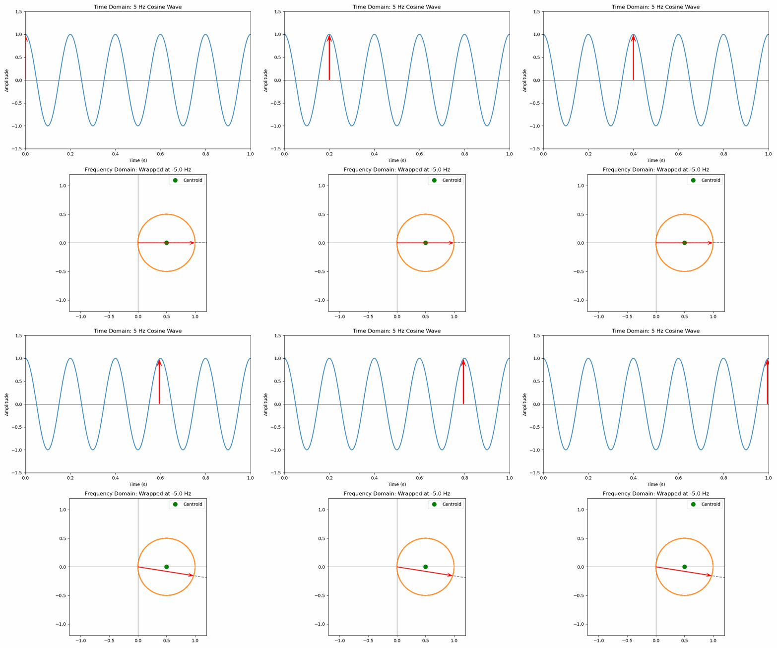Wrapping of 5Hz cosine wave at -5Hz

Notice that, for BOTH these cases - as earlier understood mathematically via Euler’s formula - the centroid of the wrapped curve is the same: equal in both magnitude and sign, both on the real axis at $A/2$.

Parallely, the REAL coordinate of the centroid in this case will look like this:

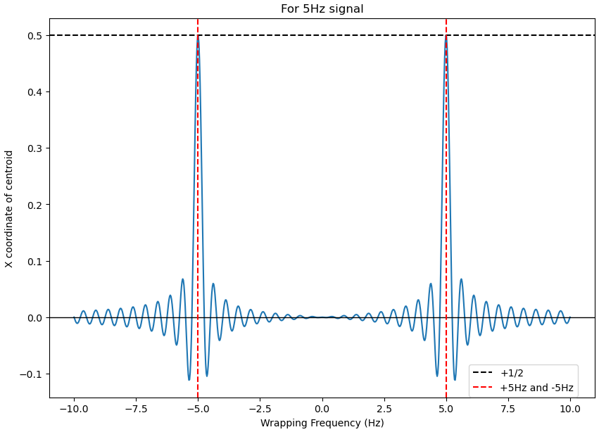X coordinate of the centroid of 5hz cosine wave wrapped at various frequencies

So, unlike the sine wave, which has equal and opposite half-amplitudes on the imaginary axis across the +/- frequency twins, the cosine wave has equal half-amplitudes on the real axis, along the conjugate frequencies.

But, what IS this “negative” frequency? Is it relevant? In the context of acoustics, at least, in the physical world, the “negative frequency” doesn’t exist as a sound you can hear. You can’t have a string vibrating -440 times per second, of course. However, in signal processing, it acts as a mathematical tool.

So yes, while it has mathematical significance, or rather, while it is a mathematical by-product of the Fourier Transform, it has no physical significance in acoustics.

3. Example case of a composite wave

From all the information we have gathered till now about the Fourier Transform, let us analyse its power by taking an arbitrary case of a composite wave. We will construct a wave from 2 different frequencies having individual phase shifts and amplitudes. The values are, respectively:

Signal 1:

• Frequency: 6Hz
• Amplitude: 1.3
• Phase shift: Advanced by 60°

Signal 2:

• Frequency: 10Hz
• Amplitude: 0.7
• Phase shift: Delayed by 30°

The composite wave would look like:

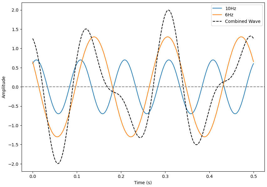Composite wave

Taking the Fourier Transform (for now, I am taking the FT values only at 6Hz and 10Hz since I know the frequency values beforehand):

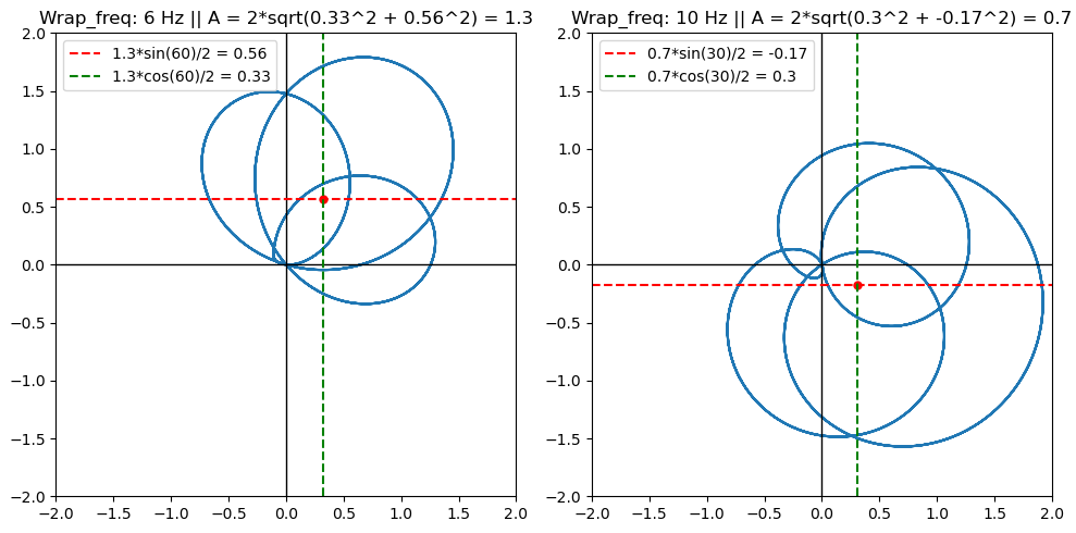Composite wave Fourier Transform

Notice how all the information of the entire composite signal is not only broken down to simple values, but also information of individual frequencies is also available, now!

• For each of the 2 frequencies, the centroid is not lying at “0”, indicating the presence of these frequencies in the composite wave.
• The entire “wrapped” shape seems rotated for both frequencies. This can be identified by the centroid, which has both real and imaginary values. You can compute the angle of the “position vector” of the centroid using the real and imaginary values, and it exactly matches the delay/advance of the PARTICULAR SIGNAL FREQUENCY present in the composite wave!
• Finally, the amplitude of the wave can be easily computed by calculating the magnitude of the complex Fourier Transform and multiplying by two!

If you have several such frequencies in the composite wave, you can simply use the Fourier Transform as a tool to extract information about these frequencies of various signals present in the wave, the amplitude of these individual signals, and also the phase information at $t=0$! This is indeed such a powerful, “entropy-reversing” tool!

But, all such tools will definitely have some shortcomings…

4. Limitations

When a signal, say an acoustic signal, is recorded or received, it is not necessary that all the frequency contents present in the time period of recording need to be present throughout the recording time frame. Perhaps a signal of frequency $f_1$ may start at a time somewhere in between the time of start of recording ($t_i$) and the end of recording ($t_f$). Or, it could also come in phases, instead of as a continuous single wave.

So, let us try out this experiment. We will pass a composite signal, which contains 2 frequency signals, with one of them “starting” at a delayed time, which is not equal to $t_i$. The signal is recorded for a total of $5\mathrm{s}$. The properties of the individual frequency signals are:

Signal 1:

• Frequency: 6Hz
• Amplitude: 0.7
• Phase: Advanced by 60°
• Start time: 0s

Signal 2:

• Frequency: 10Hz
• Amplitude: 1.3
• Phase: Delayed by 30°
• Start time: 0.7s

One second of the signal is plotted below for reference:

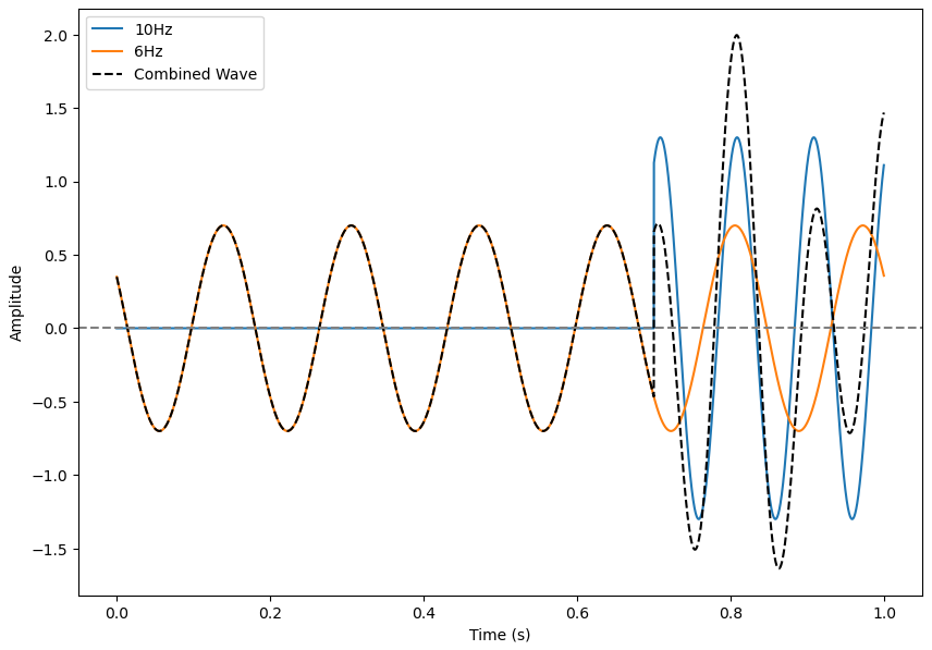Composite signal 2: 6Hz and 10Hz

Now, if the signal had BOTH the frequencies start from the time of recording itself, then you would expect the Fourier transforms to correctly predict the amplitudes of the individual frequency signals. Now, let us see the results for the above-mentioned scenario.

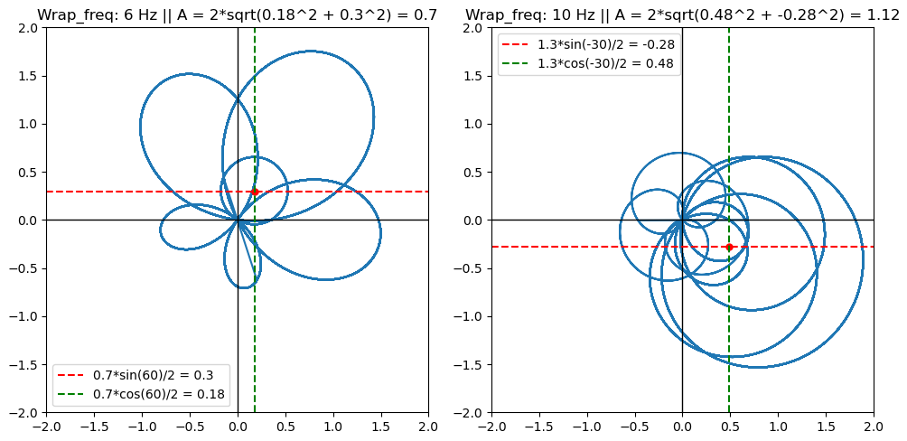Composite signal 2: Fourier Transform

The amplitude of the 6Hz wave is correctly predicted by the Fourier Transform, but what about the 10Hz wave? It is NOT 1.3 (!) The Fourier Transform is predicting the 10Hz wave to have an amplitude of 1.12, instead! Why the inconsistency here? Of course, we know it is because of the start time of this signal, since that is the only parameter being changed here. So, what changed?

This is one of the major limitations of the Fourier Transform.

Remember, I had repeatedly pointed out, that the phase of the signal being predicted by the Fourier Transform is at $t=0$ seconds. In other words, the Fourier Transform assumes that each frequency signal present in a composite wave has every frequency start right at the initial time, and end at the final time of recording. It DOES NOT store the information about the temporal distribution of each frequency wave.

Instead, it EQUALS the energy of the actual wave spread across the entire time of recording, whatever be the start or end time of signals, and spreads it across the entire temporal spectrum assuming the SAME frequency.

We will take the above case itself as an example. We will now define a “total energy” term for a particular signal.

For a signal of frequency $f$ (i.e., $f$ occurrences per second), having start and end times as $t_1$ and $t_2$ respectively, and an amplitude of $A$, the “total energy” $E$ I would like to define is:

\[E = fA\left( t_2 - t_1 \right)\]

Now, assuming the start and end time of the entire signal recording are $0$ and $t_f$ respectively, what the Fourier Transform does is equal the “total energy” $E$ across the total time $t_f$ with a wave of the same frequency but an amplitude of (say) $A_f$, i.e.,

\[E = fA\left( t_2 - t_1 \right) = fA_f t_f\]

The FFT-predicted amplitude $A_f$ is, hence:

\[A_f = \frac{fA\left( t_2 - t_1 \right)}{f t_f} = \frac{A\left( t_2 - t_1 \right)}{t_f}\]

Since $t_f$ is the maximum allowable time for a signal, it is always greater than or equal to $t_2 - t_1$, which means $A_f$ is always lesser than or equal to $A$.

In our example case,

\[A_f = \frac{A\left( t_2 - t_1 \right)}{t_f} = \frac{1.3\left( 5 - 0.7 \right)}{5} = 1.118\]

This is what is predicted in the figure as well.

This is one major limitation of the Fourier Transform. While the FT converts a signal into the frequency domain, providing a global view of all frequency components present, it loses out on all the information about when those frequencies occur. It cannot analyse signals where the frequency changes over time.

Of course, there are ways to overcome this. Typically, the Short-Term Fourier Transform (STFT) is used to overcome this by introducing time localisation. The primary mechanisms used in the STFT to introduce this temporal context are:

1. Analysis Blocks (Slicing)
2. Windowing (e.g., Hamming, Hann)
3. Overlap Factor

For now, I will close the investigation session here, and expand upon the above workarounds to tackle the major FT limitation later.

Footnotes

[1] The codes for images and animations generated by self, and even further, are consolidated here.

[2] Link for the initial, introductory post on the Fourier Transform.

_

[3] The Fourier Shift Theorem can be mathematically formulated as below:

Say for a given signal $x(t)$, the Fourier Transform is:

\[X(f) = \int_{-\infty}^{\infty} x(t)\mathbf{e}^{-j2\pi ft}dt\]

If the signal is delayed by a time $t_m$, then the delayed signal $x_m(t) = x\left( t - t_m \right)$

And the corresponding Fourier Transform is:

\[\int_{-\infty}^{\infty} x_m(t)\mathbf{e}^{-j2\pi ft}dt = \int_{-\infty}^{\infty} x\left( t - t_m \right)\mathbf{e}^{-j2\pi ft}dt\]

Substituting for a variable, $u = t - t_m$, the Fourier Transform becomes:

\[\int_{-\infty}^{\infty} x(u)\mathbf{e}^{-j2\pi f\left( u + t_m \right)}du\] \[= \mathbf{e}^{-j2\pi ft_m} \int_{-\infty}^{\infty} x(u)\mathbf{e}^{-j2\pi fu}du\]

Considering the integral term is identical to the definition of the Fourier Transform $X(f)$, only the time variable $u = t - t_m$ has replaced $t$ (these are “dummy variables” which essentially have the same function inside the integral), the Fourier Transform of the phase-shifted wave becomes:

\[\mathbf{e}^{-j2\pi ft_m} X(f)\]

The above equation represents the Fourier Shift Theorem. The exponential factor term has a function to “rotate” the “wrapped wave” (or, the wave in the frequency domain): clockwise in the frequency domain if the wave is delayed in time. Formally, a time-shift in the temporal domain becomes a multiplicative phase factor in the frequency domain.