Delay and Sum Beamforming - 3
- Introductory post on Delay and Sum Beamforming.
- Part 2 of DAS Beamforming, explaining frequency-domain DAS.
Background
In the previous two parts, we saw how a Beamformer works conceptually: first in the time domain and then in the frequency domain, using a simple demonstrative example of three signal collecting devices (here, microphones). To summarise, the working of the Beamformer array in the frequency domain goes like:
- Take the Fourier Transform of the signal recorded in each microphone. This splits the conmposite signal in each microphone into various frequency components, with both the amplitude and phase information.
- “Steer” (iterate) over various angles in the frequency domain (i.e., for each frequency signal component). For each iterating angle, calculate the time delay and recover this to advance the frequency component signal in each mic, so that the aggregate beamformer response adds constructively.
- Compute this sum of signals of all mics for a given iterator angle and the frequency component signal to obtain the aggregate array recording and response. For each frequency component, a set of responses (called Beamformer output) are obtained for each iterator angle. This is classic Delay-and-Sum Beamforming.
- For a given frequency component, the angle for which the beamformer output is maximum is the angle of incidence for that particular frequency component as per this beamformer model.
Now, even after expanding the microphone array to a complex multi-mic setup, this concept of the DAS Beamforming still iterates over angles. So, how do we get these complex heatmaps which are usually visible in Wind-Tunnel Tests of Automobiles?
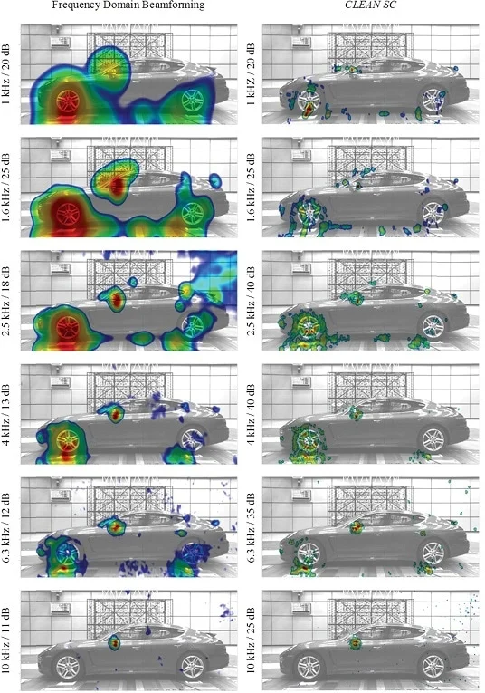 Beamforming heatmap for automobile [1]
Sound-Scanning Grid
The above heatmap is plot as a contour on a two-dimensional grid, usually parallel to the beamformer microphone array. This grid is called by various names, most commonly by “Sound Scanning Grid”. Before going deeper, let us understand the basic setup for this methodology in the case of automotive wind tunnel aero-acoustic testing.
Below is a formal setup of beamformer array in an automotive wind tunnel for aeroacoustic testing.
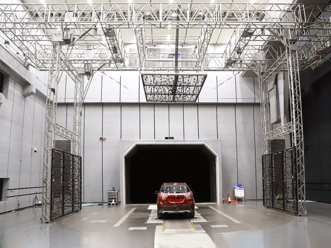 Beamforming mic setup [2]
Notice the mic setups on both the sides of the vehicle, as well as the top. The microphones are placed along a 2D plane, and their arrangements are irregular (so as to avoid Spatial Aliasing). The beamforming results from these microphone setups are plot onto a 2D Sound-Scanning Plane (SSP) which is parallel to the microphone array plane. This SSP is divided into several grids, in which the heatmmap is plot. An example setup in perspective of right-side microphone array is depicted in the below figure.
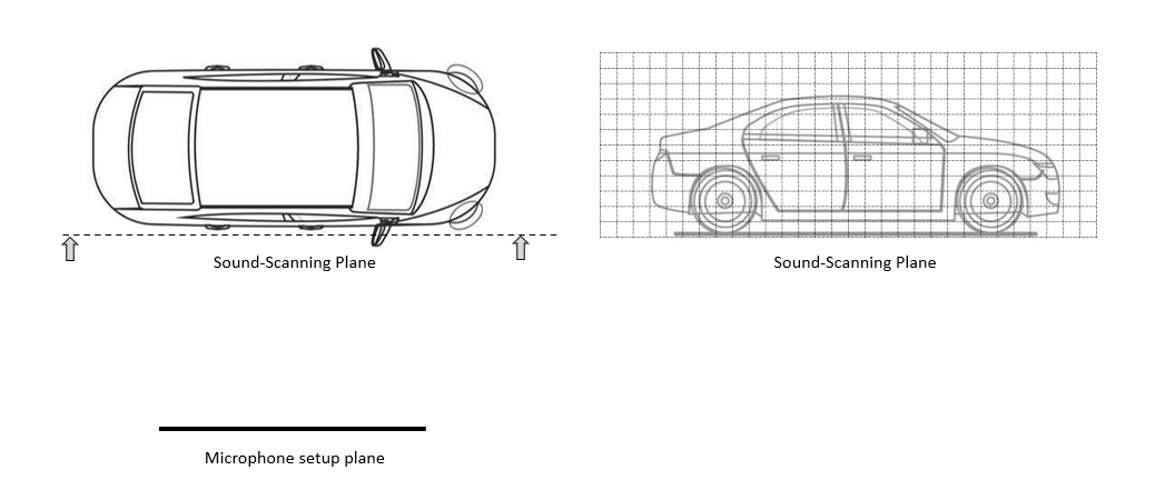 Sound-Scanning Plane Grid
In the above example, the SSP is usually placed just by the side of the car, to primarily capture the wind-noise sources from the outside rear-view-mirrors (ORVM) and the front and rear tyres. This naturally means that, the microphone array when plotting the heatmap on the grid [3], depicts the sources in that grid alone. In other words, the noise coming from the specific grid point to the microphone array setup is what is captured in this process. Hence, this mechanism is capable of capturing sound sources from anywhere in the domain; the results displayed as per the definition of the SSP. How? For this, let us go understand based on the previous two posts on beamforming.
Delay and Sum
As mentioned in the introduction of the post, the DAS works by iterating over various angles for each frequency component…
“Steer” (iterate) over various angles in the frequency domain (i.e., for each frequency signal component). For each iterating angle, calculate the time delay and recover this to advance the frequency component signal in each mic, so that the aggregate beamformer response adds constructively.
Nothing much changes in this setup, except that you now iterate over each grid point instead of just angles.
For a given frequency component, for each grid point, the distance of that grid point with each microphone is computed. Just like in the example of angular iteration, where the time delay is calculated for a given iterator angle in each microphone. If you remember the mathematical formulation, the Steering Vector for a particular frequency component and a given angle iterator and microphone $i$ is:
\[SV_i(f, \theta_0) = \mathbf{e}^{j2\pi f \left( td_i(\theta_0) \right) }\]In the above formula, the time delay $td_i(\theta_0)$ is computed for a particular iterator angle $\theta_0$, for a mic $i$. This same concept is followed in the SSP case as well. Only, the iteration is now along each pre-defined grid point, and the time delay is computed w.r.t this grid point for each microphone $i$.
The time delay for a given grid point $G$ to a mic $i$, where $D_i(G)$ is distance between the microphone and grid point, and speed of sound $c_0$, is calculated as:
\[td_i \left( G \right) = \frac{D_i(G)}{c_0}\]The Steering Vector hence for the case of SSP Beamforming becomes:
This is the modified Steering Vector [4]. Now that we have corrected for the delays, we shall do the summation. Given that the Fourier Transform (from step 1) for a given frequency component and microphone $i$ is $X_i(f)$, the corrected “advanced” signals in each mic, is thus:
\[SV_i(f, G)*X_i(f)\]The summation of this scalar, for all grid points $G$ using a Steering Vector (which has the distance between the grid point $G$ and mic $i$) for a particular frequency component $f$:
\[B(G, f) = \sum_{i = 1}^{N}\sum_{G=1}^{M} SV_i(f, G)*X_i(f)\]where $N$ is the number of microphones and $M$ is the number of grid points. Representing this in matrix format, the summation for each grid point is:
\[\begin{bmatrix} B(G_1, f) \\ B(G_2, f) \\ : \\ : \\ B(G_M, f) \end{bmatrix}_{M\mathbf{x}1} = \begin{bmatrix} SV_1(G_1, f) & SV_2(G_1, f) & ... & SV_N(G_1, f)) \\ SV_1(G_2, f) & SV_2(G_2, f) & ... & SV_N(G_2, f)) \\ : & : & ... & : \\ : & : & ... & : \\ SV_1(G_M, f) & SV_2(G_M, f) & ... & SV_N(G_M, f)) \end{bmatrix}_{M\mathbf{x}N} \begin{bmatrix} X_1(f) \\ X_2(f) \\ : \\ X_N(f)) \end{bmatrix}_{N\mathbf{x}1}\]Here, $SV_3(G_2, f)$ would mean the steering vector computes time delay w.r.t the distance of grid point 2 and microophone 3, and so on. The Fourier Transform is taken for all microphones, and hence has $N$ values for each frequency component present.
Now, remember that the Beamformer Output is (or, can be assumed as) the square of the Summation Outputs:
\[BF(G, f)_{M\mathbf{x}1} = \begin{bmatrix} \left| B(G_1, f) \right|^2 \\ \left| B(G_2, f) \right|^2 \\ : \\ : \\ \left| B(G_M, f) \right|^2 \end{bmatrix}_{M\mathbf{x}1}\]This beamformer output $BF(G, f)$ has $M$ values corresponding to each grid point, which is plot as the heatmap for that particular frequency.
Beamformer Output for a frequency range
Sometimes we have to show this heatmap over a range of frequencies (like 1kHz - 2kHz). In which case, we need to aggregate the Beamformer Output of shape Mx1 of different frequency components. To aggregate this output, we shall use the “Frequency Resolution” of the (Discrete) Fourier Transform, $\Delta f$ [5].
If say the lower limit of frequency required in the heatmap is $f_1$,a nd the higher limit is $f_2$, then the discrete frequency components present in the DFT are:
\[f_1, \qquad f_1 + \Delta f, \qquad f_1 + 2\Delta f, \qquad ..., \qquad f_2 - \Delta f, \qquad f_2\]Which means, we shall have (from the above DAS Beamformer), the following outputs:
\[BF(G, f_1), \qquad BF(G, f_1 + \Delta f), \qquad BF(G, f_1 + 2\Delta f), \qquad ..., \qquad BF(G, f_2 - \Delta f), \qquad BF(G, f_2)\]all of which have shape $M\mathbf{x}1$.
The aggregate Beamformer Output between these frequency ranges is defined as:
\[BF(G) \left[ f_1, f_2 \right] = \Delta f \sum_{f_a = f_1}^{f_2}BF(G, f_a)\]This is an energy summation, called the Riemann Sum Approximation. Sometimes, the above summation is also normed according to the number of microphones $N$:
\[BF(G) \left[ f_1, f_2 \right] = \frac{\Delta f}{N^k} \sum_{f_a = f_1}^{f_2}BF(G, f_a)\]where $k$ is the norm power. One could use a $k$ value of 1 for dampening of the sound source magnitudes, or a value of 0.5 for slight amplification.
Keep in mind that the unit of the above output is $\mathbf{Pa}^2$, due to the squaring during the Beamformer output computation step. The base unit of $\mathbf{Pa}$ is from the Fourier Transform $X_i(f)$. So, if I want to show the above aggregated Beamformer output in decibels:
\[BF(G)_{dB} \left[ f_1, f_2 \right] = 10\mathbf{log}_{10}\left( \frac{BF(G) \left[ f_1, f_2 \right]}{p_{ref}} \right)\]where $p_{ref}$ is 2E-5 $\mathbf{Pa}$ for air.
This beamformer output in decibels has as many values as there are grid points. This can be plot as a contour on the SSP [6]. Also, all the matrix multiplications and handling of mic and grid arrays can be done efficiently in Python [7].
All this should make one thing clear: the Beamformer output, even in dB, is not indicative of the actual noise heard in the noise sources, but is good for a comparative analysis of noise sources provided all the parameters in the computation are kept the same.
Constand Beamwidth DAS Beamforming
Effective aperture
In microphone arrays, the overall size or spatial span of the entire array dictates the array’s spatial resolution. It is called the physical aperture of the array. Mathematically, it is the distance between the outermost microphones in the array. In circular or semi-circular arrangement of microphones, it is generally the diameter of the entire setup. Let us called the Physical Aperture by $A_p$.
For a given microphone array, the physical aperture remains constant. However, the acoustic waves don’t “see” in meters. They interact based on their wavelength. For this, the Acoustic Aperture $A_a$ is defined, which is a measure of the array aperture relative to the measuring frequency, i.e., it is what the particular frequency component “sees”. Mathematically:
\[A_a = \frac{A_p}{\lambda}\]Now, for a high frequency wave, it contains higher number of waves (defined by the time period) in a fixed length than a low frequency wave. That means, for a given physical aperture, the acoustic waves “see” this aperture as “bigger” due to presence of multiple waves with respect to a lower frequency wave. This is defined by the acoustic aperture.
The Spatial Resolution of an array is defined as the reciprocal of the Acoustic Aperture. It is called the Beamwidth $\theta_b$, it defines how narrowly the array can focus its “beam” to poinpoint a specific noise source.
\[\theta_b = \frac{\lambda}{A_p} = \frac{c_0}{f.A_p}\]where $c_0$ is the speed of sound. Since $c_0$ and $A_p$ are constants, the beamwidth is entirely dependent on the frequency of the wave. Which means:
- Higher Frequencies: The fixed physical aperture spans many wavelengths. The array is “acoustically large” (high acoustic aperture). This produces a very narrow beamwidth, giving you sharp, high spatial resolution.
- Lower Frequencies: The exact same physical aperture might span only one or two wavelengths. The array is “acoustically small”. The resulting beamwidth is wide and blurry, resulting in poor spatial resolution.
This can be understood with photographic analogy as well. A larger acoustic aperture and smaller beamwidth behaves like a highly focused telephoto lens, easily isolating and pin-pointing high frequency sources. While a wider beamwidth acts like a wide-angle lens, providing lower resolution but capturing a larger area. A low frequency dipole source will look like a big blob in the beamforming heatmap when compared to the higher frequency resolution.
This is pictorially represented in the dynamic plot below. It shows the DAS algorothm applied for a particular frequency wave. For now I have selected (randomly) 51 microphones for this output. The Boresight is the angle measured w.r.t the array perpendicular normal coming out of the center of the array. When you slide the frequency or the aperture to the right, you will see $D/\lambda$ increase and the dispersed “main lobe” instantly narrow, thus improving the acoustic resolution.
Hence, there is this inherent “bias” towards higher frequencies when it comes to spatial resolution [8]. To overcome this bias, we need a constant resolution across frequencies, a constant beamwidth. A constant Beamwidth is obtained by using Frequency-dependent Spatial Weighting, in which we intentionally “cripple” the high frequency resolutions.
Another disadvantage you can notice here is the presence of Sidelobes, which degrade the spatial selectivity by allowing unwanted signals from other angles to leak into the system. This too has to be addressed during frequency weightage.
Frequency-dependent Weighting
Essentially, what it does is:
- At low frequencies: The system uses all the microphones, utilizing the entire physical aperture ($A_p$) to get the best possible narrow beam.
- At high frequencies: The system mathematically “turns off” the outer rings of microphones. This physically shrinks the active aperture ($A_p$) as the frequency climbs.
By shrinking $A_p$ exactly as fast as $\lambda$ shrinks, we maintain a constant beamwidth $\lambda/A_p$. The result being: the array gives the exact same (blurry) resolution at (say) 10kHz that it gives you at 1kHz. You lose your high-frequency pinpoint accuracy, but you gain a consistent beamwidth across the entire spectrum. This is formally called Constant Beamwidth (Delay and Sum) Beamforming (CBB) or Frequency-invariant beamforming (FIB).
Mathematically, it is achieved by applying frequency-dependent weightage (also called frequency-dependent spatial shading (let us call it FDSS)) to the microphones. Specifically, this FDSS is applied on to the Steering Vector function, to shrink the active size of the array mathematically as the frequency increases.
As we established, the beamwidth is inversely proportional to the frequency and the physical aperture. Since we are now dealing with activating or de-activating microphones based on frequencies, we will call this the active physical aperture, $A_{pa}$.
\[\theta_b \propto \frac{c_0}{f \cdot A_{pa}}\]To force the beamwidth to be constant across all frequencies, we must enforce an inverse relationship between the active aperture and the frequency:
\[A_{pa} \propto \frac{1}{f}\]This is achieved by applying a weighting vector $\mathbf{w}(f)$ to the mirophones. Let $r_i$ be the radial distance of the $i$-th microphone from the array center. The weighting function should be such that, it is wide at low frequencies (using all mics) and narrow at high frequencies (virtually turning off the outer mics).
A standard choice is a frequency dependent Gaussian Shading [9], which also handles Sidelobes [10]:
\[w_i(f) = \exp \left( - \frac{r_i^2}{2 \sigma(f)^2} \right)\]And the vector $\mathbf{w}(f) = \begin{bmatrix} w_1(f) & w_2(f) & .. & w_N(f) \end{bmatrix}$. To satisfy the constant beamwidth condition, the standard deviation $\sigma(f)$ is set to scale inversely with the frequency:
\[\sigma(f) = R_{\text{max}} \frac{f_{\text{ref}}}{f}\]where, $R_{\text{max}}$ is the physical radius of the array (the maximum of all $r_i$), and $f_{\text{ref}}$ is a chosen reference frequency (usually the lowest frequency of concern, where the entire array is active).
The weightage distribution for a mic array with radius $r_{\text{max}}$, reference frequency for weightage $f_{\text{ref}}$ and frequency of processing wave $f$ is shown below:
Note that, if you set the “ceiling” reference frequency as say 2kHz, then increasing the operating frequency increases the rate of decay of weight towards the outer regions of the microphone array (i.e., $\pm r_{\text{max}}$). For example, for $f$ = 4000 Hz, the weightage given to the outer ring of mics is only about 13%.
Now we will apply this Gaussian Shading and visualise the Beamwidth, compare both the Constant Beamwidth and Standard DAS Beamforming methods:
Notice this: when you drag the Operating Frequency slider above the Reference Frequency (e.g., leaving $f_{\text{ref}}$ at 2000 Hz and sliding $f$ up to 8000 Hz), you will notice that the Standard DAS Beamwidth becomes incredibly narrow, representing the bias as discussed earlier. However, the Gaussian Weighted CBB Beamwidth will maintain almost the exact same main lobe width it had at 2000 Hz.
Frequency-dependent weighting to remove Sidelobes
There are two different observations here, depending on whether operating frequency is above or below the reference frequency:
Above $f_{\text{ref}}$: The “Constant Beamwidth” Regime: As explained above, the “main lobe” is exactly the same in this region, whatever is the operating frequency. The goal here is to have the same target resolution across all frequencies. Here, you have more than enough microphones due to the small wavelength of waves. Also, due to the Gaussian Weightage, the sidelobes are naturally supressed [10].
Below $f_{\text{ref}}$: The “Sidelobe Suppression” Regime: Here, due to the long wave lengths, the effective (acoustic) aperture is significantly smaller than the previous case, and hence the main lobe is going to get inevitably wider. That is a consequence of both DAS Beamforming and its tweaks including CBB, which cannot be overcome. In addition to that, the sidelobes are now massive. To understand this, play around with the Gaussian weight interactive chart: say, choose reference frequency of 2000Hz and operating frequency of 500Hz. In this case, the Gaussian weights at the outermost mics (at $r_{\text{max}}$) is still 96%! It is essentially a rectangular weightage now. On applying the DAS algorithm (and consequentially the Fourier Transform), the sidelobes appear again.
For the first limitation (of poorer resolution), there is simply no solution other than to increase the aperture size to capture with high resolution the larger wavelengths.
For the sidelobe removal, the Gaussian Weightage should not be allowed to become rectangular once the operating frequency drops significantly below the reference frequency. This can be achieved by locking the standard deviation of the Gaussian curve as soon as the operating frequency approaches the reference frequency. I shall call this the Floor-Locked Frequency Weightage [11].
As mentioned earlier, the Gaussian Shading:
\[w_i(f) = \exp \left( - \frac{r_i^2}{2 \sigma(f)^2} \right)\]where
\[\sigma(f) = R_{\text{max}} \frac{f_{\text{ref}}}{f}\]Here, we need to lock down $\sigma$ when operating frequency decreases below reference frequency, such that sigma is a constant below this range. Essentially, the idea is to keep the ratio of $f_{\text{ref}}/f \ge 1$. Thus, the floor-locked frequency weightage is defined by a modified $\sigma$:
\[\sigma(f) = \left\{ \begin{aligned} &R_{\text{max}} \frac{f_{\text{ref}}}{f} \qquad &&\text{if} \quad f>f_{\text{ref}} \\ &R_{\text{max}} &&\text{if} \quad f \leq f_{\text{ref}} \end{aligned} \right.\]Now, we will visualise how this floor-locked frequency weightage is distributed as before:
The corresponding Beamwidth resolution using the DAS algorithm:
Let us again analyse the two frequency regions:
For operating frequencies above the reference frequency, the frequency weightage is the same and hence so is the Beamwidth resolution output from the DAS beamformer: constant resolution for all frequencies with no side-lobes, both due to Gaussian Shading. The Constant resolution due to compensation of resolution at higher frequencies by lesser weightage for outer microphones, and no side-lobes due to the Gaussian weightage providing a smooth transition of weights from outermics to free-air (0 weight)
For operating frequencies below the reference frequency, the Floor-Locked Frequency weightage has a constant Gaussian curve, thus eliminating the Rectangular transition of weights in the case of “Unlocked” Frequency weightage. This causes a Gaussian-ish Fourier Transform as well, thus removal of side-lobes in the Floor-Locked frequency weightage case.
I think this is enough “exploration” for now. This has produced reasonably good results at my end (okayish at values, excellent heatmap pattern match [12]), though I cannot show the same due to confidentiality. The code though, has been entirely developed by me in my personal time, and hence the liberty to reproduce them here.
Footnotes
[3] The grid spacing, plane location, plane length and width, can all be standardized or chosen based on the needs/requirements of testing, expected results and overall vehicle development.
[4] Keep in mind that the exponent here has no negative sign, due to the time advancement discussed in the earlier post. To summarize: the signal received by a given microphone is assumed to have a time delay (say with respect to a “base” mic):
\[s_i(t) = s_b \left( t - td_i \right)\]In the frequency domain, the above time delay is a negative exponent.
Now, to have constructive interference, we ADD the time delay and ADVANCE the signal in mic $i$, such that the newly computed “advanced” signal in mic $i$:
\[sa_i(t) = s_i \left( t + td_i \right) = s_b (t)\][5] In Digital Signal Processing, the Fourier Transform computed is always the Discrete Fourier Transform. Which means that, the output FT is not a continuous function of the frequency, but has discrete frequency values in which the FT exists. The minimum frequency resolution (i.e., the difference between any two frequency values in the DFT) is ditrectly dependent on the sampling frequency and the total number of samples recorded. The frequency resolution is given by:
\[\Delta f = \frac{f_s}{N}\]Some observations are:
- If the sampling frequency $f_s$ is increased keeping the total number of samples $N$ constant (i.e., the total time of recording decreased), then the frequency resolution $\Delta f$ decreases.
- If the total number of samples is increases keeping the sampling frequency constant (i.e., increase the total time of recording), then the frequency resolution increases.
Which naturally means, recording for a longer period is better for getting highly resolved Fourier Transforms.
[6] Plotting as a contour can be easily done in Python by the following code:
1
plt.contourf(bfmap) # Make sure bfmap is of shape (ny, nx)
[7] Some examples of efficient coding for swift results:
1
2
3
4
5
6
7
8
9
10
11
12
13
14
15
16
17
18
19
20
21
22
23
24
25
26
27
28
29
30
31
32
33
'''For Distance computation'''
D = np.linalg.norm(G[:, None, :] - P[None, :, :], axis = 2)
# G is grids, of shape (ny*nx, 3). By doing G[:, None, :], you convert it to shape (ny*nx, 1, 3)
# P is mics of shape (nm, 3). By doing P[None, :, :], you convert it to shape (1, nm, 3)
# Such that D is of shape (ny*nx, nm)

'''For FFT storage'''
FFT_mat = np.zeros((len(freqs), len(P)), dtype = np.complex128) # freqs are values of all frequencies of DFT required. Hence, shape is (nf, nm)
for m in range(len(P)):
	FFT_mat[:, m] = df[m] # df has all frequency DFTs, for every mic.

'''DAS Beamforming'''
def steering_vect(f):
	c0 = 343
	expo = -1j*2*np.pi*f*D/c0 # Just input D which has all distances for a particular frequency, of shape (ny*nx, nm)
	return np.exp(expo) # Hence SV also has shape (ny*nx, nm)

bf_tots = []
for i, f in enumerate(freqs):
	SV = steering_vector(f) # (ny*nx, nm)
	X = FFT_mat[i]
	#BF output for ALL grid points at once
	bf_vals = np.abs(SV.conj() @ X)**2 # conjugate of SV for time advancement as explained earlier, since steering vector is computed for a time delay. Also, shape is (ny*nx, nm).(nm,) = (ny*nx)
	bf_tots.append(bf_vals)
bfarr = np.array(bf_tots)

bfdb_grid = []
for i in range(G):
	normed = (deltaf/len(P)**1)*bfarr[:, i].sum() # Aggregated for all frequency for a particular grid point
	pref = 20E-6
	bfdb = 10*np.log10(normed/pref**2)
	bfdb_grid.append(bfdb)
bfmap = np.array(bfdb_grid).reshape(ny, nx)
This is to the extent of the code which I am comfortable in reproducing in public. The rest is.. well.. locked away, personal reasons.
[8] The microphone arrays have two geometric constrains:
- Low Frequency Floor: At lower frequencies (higher wavelengths), if the wave is longer than or roughly equal to the entire width (physical aperture) of the array, the resolution becomes so wide and blurry that the array cannot distinguish whether (say) a noise is coming from the ORVM or the A-pillar.
- High Frequency Ceiling: As the acoustic aperture gets larger and larger, the resolution gets sharper and the bias gets higher for higher frequencies. However, this “bias” hits a wall for a fixed array setup: Spatial Aliasing). Once a single half wave-length of the high frequency wave gets below the distance between your adjacent microphones, or $\lambda/2 < d$, then the spatial Nyquist Criteria is crossed. In this case, a half wave is able to fit inside or within the microphone spacing, thus causing the array setup to read the signals for what they may not be, just as in temporal aliasing. The array will confidently pinpoint loud noise sources at particular frequencies and locations, both of which may not exist in reality. Hence, to avoid this, we have to push the mics closer together.
[9] A Gaussian weightage is ideal for such scenarios where there is radially dependent weightage, with the maximum weightage at the center. $e^x$ has exponential growth, $e^{-x}$ has exponential decay, and $e^{-x^2}$ follows a “normal” distribution centered at zero.
The Standard Deviation is defined as $\sigma$, such that for a normal distribution following $e^{-x^2/2\sigma^2}$, the points at $x = \pm \sigma$ are the inflection points where the Gaussian curves change concavity. The area under $x = \pm \sigma$ of the Gaussian curve w.r.t the total area under the curve is also a fixed constant at ~68.2%. See below
Since our goal is to reduce weightage when moving away from the array center, this is an ideal function. Here, $\sigma$ decides how fast the weights decay with radius. As frequency increases, progressively ignore microphones farther from the center.
[10] Sidelobes are present in the CBB output because of the Fourier Transform. By default, the Delay-and-Sum beamforming has equal weightage to all microphones. On performing the DAS algorithm which includes the Fourier Transformation, a rectangular window is applied wherein there is a sudden drop in weight from 1 to 0 (of the surroundings). And the Fourier Transform of a rectangular wave is $\mathbf{sin}(x)/x$, which inherently has such “side-lobe” kind of structures.
But when applying a pure Gaussian weightage where the weights smoothly transition to 0 of the surroundings from the outermost mics, the Fourier Transform does not contain any side lobes. This is because the Fourier Transform of a purely Gaussian is also a Gaussian!
[11] The Python code for this “floor-locked frequency weightage” in Python is applied to the steering vector. The same code as [6] is used here too, but the steering vector is tweaked:
1
2
3
4
5
6
7
8
9
10
11
12
13
r_mics = np.sqrt(P[:, 0]**2 + P[:, 1]**2) # P is mic coordinates. Assuming it is in the z plane, this is simply the position of each mic, r_i in the formula
r_max = max(r_mics)
def steering_vect(f):
	c0 = 343
	expo = -1j*2*np.pi*f*D/c0
	fref = 2000 # (Say)
	if f > fref:
		sigma = (fref / f) * (r_max) # Idea is, ratio of (fref/f) should never be less than 1
	else:
		sigma = r_max
	weights = np.exp(-((r_mics/sigma)**2)/2)

	return np.exp(expo)*weights
[12] Do note that to reproduce the result accuracy in terms of values with commercial and well-established softwares, it requires complete knowledge of the settings and parameters and algorithms they use. No doubt, they probably use even more sophisticated algorithms to counter the many more limitations of the above explained Beamforming algorithm. Furthermore, the parameters I have used, the assumptions I have taken, may not be the same as what commercial softwares use, most of which is not possible for me to know due to confidentiality anyway. But the very fact that heatmap contours are matching exactly is a great encouragement for me, since it means I am atleast right in my code.