RANS First-Order Turbulence Models
RANS
To model turbulence, one method is by Reynolds Averaging the Navier-Stokes equations which leads to the Turbulence Closure Problem in the RANS equations (as discussed here). RANS equations are given by:
\[\frac{\partial \overline{u_i}}{\partial t} + \overline{u_j} \frac{\partial \overline{u_i}}{\partial x_j} = -\frac{1}{\rho} \frac{\partial \overline{p} }{\partial x_i} + \nu \frac{\partial^2 \overline{u_i}}{\partial x_j^2} - \frac{\partial \overline{u_i^{\prime}} \overline{u_j^{\prime}} }{\partial x_j}\]RANS can be solved by various methods, one of which is modeling the Reynolds Stress Tensor directly and is hence called First-Order Models.
First-Order Models are modeled based on the assumption of similarity of the structure of the stress tensor between laminar and turbulent flows, i.e., based on an analogy between them. The stress tensor for laminar flows for Newtonian fluids is familiar to us:
\[\tau_{ij} = \nu \left( \frac{\partial u_i}{\partial x_j} + \frac{\partial u_j}{\partial x_i} \right) - \frac{2}{3}\nu\frac{\partial u_k}{\partial x_k}\delta_{ij} = 2\nu S_{ij} - \frac{2}{3}\nu\frac{\partial u_k}{\partial x_k}\delta_{ij}\]where $\delta_{ij}$ is the kronecker delta and $S_{ij}$ is the Strain-Rate Tensor. For incompressible flows, the final term becomes zero due to continuity equation.
\[\tau_{ij} = 2\nu S_{ij}, \qquad S_{ij} = \frac{1}{2} \left( \frac{\partial u_i}{\partial x_j} + \frac{\partial u_j}{\partial x_i} \right)\]Boussinesq Hypothesis
In First-Order Models, it is hypothesised that, the Reynolds Stress Tensor has the same structure as the above case. For RST, the symbol of $\tau$ is used, since it is a tensor and hence symbolising shear.
\[\tau_{ij}^{turb} = -\overline{u_i^{'}u_j^{'}} = 2\frac{\mu_t}{\rho} S_{ij} - \frac{2}{3} \delta_{ij}k \ , \quad S_{ij} = \frac{1}{2} \left( \frac{\partial \overline{u_i}}{\partial x_j} + \frac{\partial \overline{u_j}}{\partial x_i} \right)\]It can be noticed here that the RST containing instantaneous velocities (and 6 unknown terms) is written in terms of the mean flow variables, a scalar quantity known as turbulent viscosity or eddy viscosity, and the (specific) Turbulent Kinetic Energy. The purpose of these turbulence models is to compute this turbulent viscosity to get around the closure problem.
This particular hypothesis of relating the RST as a factor of the Strain Rate Tensor is called the Boussinesq Hypothesis. For Non-Newtonian fluids, the Boussinesq hypothesis has non-linear relation of the turbulent shear stress with the Strain tensor
Turbulent Diffusion
- Why is a “viscosity” chosen as the proportionality constant? Because, turbulence by its nature is dissipative, but this dissipation is NOT molecular diffusion.
- Turbulence is characterized by high Re and hence high inertial force over viscous force, thus the molecular diffusion is indeed very minute in comparison to advection or inertial force.
- But turbulence IS dissipative. This diffusion is called turbulent diffusion, and is (hence, here) mathematically represented by the turbulent viscosity. Infact, this mathematical assumption when substitued in the RANS term, the diffusion term becomes:
Notice how the diffusion term is increased via the addition of the turbulent viscosity term.
Since this parameter is a mathematical concept to be used for CFD to manifest directly the dissipative propoerty of turbulence, it is NOT a propoerty of the fluid, but is a property of the FLOW.
More on the Boussinesq Hypothesis
The Boussinesq Hypothesis is a “brutal and flawed” approximation of the actual physics, but it has been demonstrated that it is accurate if good standard practices are followed. It can be noticed above that the hypothesis contains a term proportional to the (specific) Turbulent Kinetic Energy for the principal components of the stress tensor (as represented by the kronecker delta). The significance of it is for consistency.
The RST is given by:
\[\begin{equation} \tau_{ij}^{turb} = -\overline{u_i^{\prime}} \overline{u_j^{\prime}} = - \left(\begin{array}{lll} \overline{u^{\prime} u^{\prime}} & \overline{u^{\prime} v^{\prime}} & \overline{u^{\prime} w^{\prime}} \\ \overline{v^{\prime} u^{\prime}} & \overline{v^{\prime} v^{\prime}} & \overline{v^{\prime} w^{\prime}} \\ \overline{w^{\prime} u^{\prime}} & \overline{w^{\prime} v^{\prime}} & \overline{w^{\prime} w^{\prime}}\end{array}\right) \label{eq:1} \end{equation}\]As per the Boussinesq Hypothesis:
\[\begin{equation} \tau_{ij}^{turb} = 2\frac{\mu_t}{\rho} S_{ij} - \frac{2}{3} \delta_{ij}k = \frac{1}{\rho} \left(\begin{array}{lll} 2\mu_t S_{11} - \frac{2}{3}k & 2\mu_t S_{12} & 2\mu_t S_{13} \\ 2\mu_t S_{21} & 2\mu_t S_{22} - \frac{2}{3}k & 2\mu_t S_{23} \\ 2\mu_t S_{31} & 2\mu_t S_{32} & 2\mu_t S_{33} - \frac{2}{3}k\end{array}\right) \label{eq:2} \end{equation}\]where,
\[S_{11} = \frac{\partial u_1}{\partial x_1}, \quad S_{12} = \frac{1}{2}\left( \frac{\partial u_1}{\partial x_2} + \frac{\partial u_2}{\partial x_1} \right) \quad \mathrm{etc.}\]Taking the trace of tensor in \eqref{eq:1}:
\[\tau_{ii}^{turb} = -\left( \overline{u_1^{\prime2}} + \overline{u_2^{\prime2}} + \overline{u_3^{\prime2}} \right)\]Taking the trace of tensor in \eqref{eq:2}:
\[\tau_{ii}^{turb} = 2\nu_t\left(\frac{\partial u_i}{\partial x_i}\right) - 2k = -2k\]Equating the above two:
\[k [m^2/s^2] = \frac{1}{2}\left( \overline{u_1^{\prime2}} + \overline{u_2^{\prime2}} + \overline{u_3^{\prime2}} \right)\]Which is consistent with the definition of (specific) TKE; hence the significance of the last term in the Boussinesq Hypothesis.
This Hypothesis is the most commonly used method to model turbulence. Although, it does have a limitation in that it assumes an isotropic scalar quantity in the turbulent viscosity $\nu_t$. There are several models which treat it as anisotropic quantity or a tensor (tensors can capture anisotropy, vectors can’t fully only partially).
Either way, in order to compute the turbulent viscosity from it, various models are used:
First-Order RANS Turbulence Models
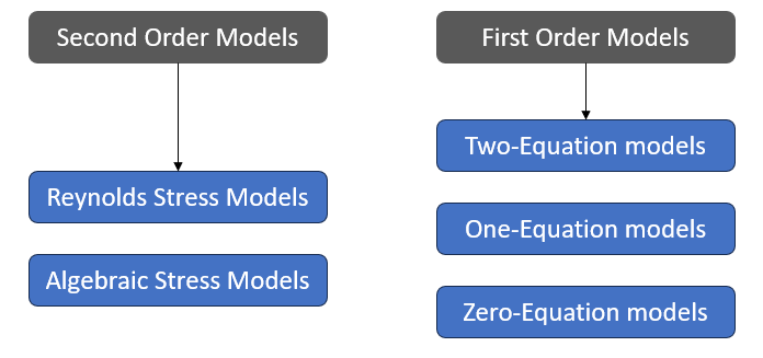 Reynolds Averaging Turbulence Models
1. Zero-Equation Models
These are based on the Mixing Length Theory and simple Dimensional Analysis. Here, the turbulent viscosity is assumed as being proportional to the turbulent length scale times the turbulent velocity scale.
\[\nu_t \left[ m^2/s \right] = l_s \left[ m \right]*u_s \left[ m/s \right]\] \[\nu_t = l_o * l_o \frac{dU}{dy}\]where $l_o$ is the mixing length used as the length scale.
The Mixing Length is determined from experiments or the Boundary Layer Theory. Although, it should be noted that $l_o$ is NOT universal and depends on the nature of the problem.
Pros
- Easy to implement
- Fast
- Accurate for simpler flows where $l_o$ is determined experimentally
Cons
- When $l_o$ is unknwon (which is most engineering problems), results are very inaccurate. Especially for flows with separation or re-circulation.
2. One-Equation Models
The guess for the velocity scale in the mixing length model of the Zero-Equation model can be improved further. It can be characterized using the (specific) Turbulent Kinetic Energy.
\[u_s = \sqrt k\]where,
\[k = \frac{1}{2} \overline{u_i^{\prime}} \overline{u_i^{\prime}}\]But again, we do not know $u_i^{\prime}$. Hence an equation for TKE is directly developed. But it is still dependent on the mixing length scale (not shown here)
3. Two-Equation models
These models are used to overcome the non-universality limitation of the length scale present in the previous two models. A more universal quantity is to be used to scale the turbulent viscosity. For this, the three important quantities in the energy cascade - turbulent viscosity ($\mu_t$), Turbulent Kinetic Energy ($k$), and Turbulence Dissipation Rate ($\epsilon$) - are related together via simple dimensional analysis.
\[\nu_t \propto l_su_s\] \[\nu_t \left[ m^2/s \right] \propto \frac{k^2}{\epsilon} \left[ \frac{m^4/s^4}{m^2/s^3} \right]\] \[\begin{equation} \nu_t = C_\mu\frac{k^2}{\epsilon} \label{eq:3} \end{equation}\]Turbulent Kinetic Energy alone does not distinguish between large and small eddies. For this, Turbulence Dissipation Rate is used.
\[\epsilon = \nu \overline{\frac{\partial u_i^\prime}{\partial x_j} \frac{\partial u_j^\prime}{\partial x_i}}\]Again, $u^\prime$ is unknown. Hence, transport equations are developed for both $k$ and $\epsilon$ from the Navier-Stokes equations. The final $k-\epsilon$ model for incompressible flows with all the equations are (Momentum equation derived using the Boussinesq Hypothesis, as before)
\[\frac{\partial \overline{u_i} }{\partial x_i} = 0\] \[\frac{\partial \overline{u}_i}{\partial t} + \overline{u_j} \frac{\partial \overline{u}_i}{\partial x_j} = - \frac{1}{\rho} \frac{\partial \overline{p}}{\partial x_i} + \frac{\partial}{\partial x_j} \left[ \left( \nu + \nu_T \right) \frac{\partial \overline{u}_i}{\partial x_j} \right] - \frac{2}{3} \frac{\partial k}{\partial x_i}\] \[\frac{\partial k}{\partial t} + \overline{u_j} \frac{\partial k}{\partial x_j} = \frac{\partial}{\partial x_j}\left[ \left( \nu + \frac{\nu_T}{\sigma_k} \right) \frac{\partial k}{\partial x_j} \right] + P - \epsilon\] \[\frac{\partial \epsilon}{\partial t} + \overline{u_j} \frac{\partial \epsilon}{\partial x_j} = \frac{\partial}{\partial x_j}\left[ \left( \nu + \frac{\nu_T}{\sigma_{\epsilon}} \right) \frac{\partial \epsilon}{\partial x_j} \right] + C_{\epsilon_1} \frac{P \epsilon}{k} - C_{\epsilon_2} \frac{\epsilon^2}{k}\] \[\nu_T = C_{\mu} \frac{k^2}{\epsilon}\]where,
\[P = -\overline{u_i^\prime u_j^\prime}\frac{\partial \overline{u_i}}{\partial x_j}, \quad \epsilon = \nu \overline{\frac{\partial u_i^\prime}{\partial x_j} \frac{\partial u_j^\prime}{\partial x_i}}\]and the constants for this model are (as obtained from experiments):
\[C_{\mu} = 0.09, \quad C_{\epsilon_1}=1.44, \quad C_{\epsilon_2}=1.92, \quad \sigma_{\epsilon}=1.3, \quad \sigma_k = 1\]In the RHS of the $k$ and $\epsilon$ transport equations, the terms are: Turbulent Transport + Production + Dissipation. The last two terms are source terms.
- In the CFD simulations using $k-\epsilon$ models, two iterative loops are present as part of the solution methodology.
- The first one involves solving for the $k$ and $\epsilon$ transport equations with the previous iteration or initial condition of the unknown variables; computing the turbulent viscosity and then solving the momentum equations.
- When solving the momentum equations, the Pressure-Velocity coupling is encountered, for which another iterative procedure is deployed involving the Pressure-Possion Equation (say). Hence, in every time step, double-nested iterative loops are present.
Pros
- Easy to implement
- Stable calculations and overall good predictions
- Useful for free shear layer flows with small pressure gradients (best in the free stream)
Cons
- Poor predictions for flows with high and adverse pressure gradients, like
- Swirling/Rotating flows
- Separations
- Axisymmetric jets
- Non-circular ducts
- Near-wall issues (as $k \to 0$ near wall)
The k-omega turbulence model
Similarly, the the governing equations of the $k-\omega$ model is derived, where $\omega$ is the specific rate of dissipation of TKE (units $1/s$). It can be thought of as:
- Reciprocal of $\omega$ gives time scale of turbulence dissipation
- It gives the rate at which turbulence is dissipated to smallest eddies
- It is some frequency at which the eddies are dissipated.
The turbulent kinematic viscosity in terms of the specific rate of TKE dissipation ($\omega$) is given as:
\[\nu_t = \frac k \omega\]Hence (at least as per OpenFOAM):
\[\begin{equation} \omega = \frac{\epsilon}{C_\mu k} \label{eq:4} \end{equation}\]This model is:
- Very accurate for 2D boundary layer flows with both favourable and adverse PGs
- Can be easily integrated through the viscous sublayers
- But unfortunately, it is sensitive to free stream Boundary Conditions.
One such turbulence model which combines both the $k-\epsilon$ and $k-\omega$ turbulence models is the SST k-omega, which has a blended function wherein the k-epsilon is applied in the free-stream, and the k-omega is triggered near wall.
Turbulent Length Scale
The Turbulent Length Scale does not appear explicitly in the CFD solution. It is used to assign a value for $k$ and $\epsilon$ at the boundaries, and for their initial conditions which are not known a priori. The Turbulent Length scale is typically estimated as a fraction of the domain’s characteristic dimension. Foe example, for fully developed pipe flows, it can be estimated from the hydraulic diameter, (typically, ~3.8%). For codes using a Turbulence Length-scale based on the mixing-length (Fluent, OpenFOAM) 3.8% is replaced with 7%.
\[\begin{equation} l_s = 0.07d_h \label{eq:5} \end{equation}\]The TKE is specified as:
\[\begin{equation} k = \frac 1 2 \left( u^{\prime 2} + v^{\prime 2} + z^{\prime 2} \right) \approx \frac{3}{2}(U_{rms}^{\prime})^2 \label{eq:6} \end{equation}\]where $U_{rms}^\prime$ is the Root mean square of the velocity fluctuations. The assumption of equality of fluctuating velocities in all directions holds good for an initial/boundary guess. The RMS velocity can be expressed in terms of Turbulent Intensity ($I$)
\[\begin{equation} U_{rms}^{\prime} = IU_\infty \label{eq:7} \end{equation}\]$I$ can be written generally in terms of the Reynolds Number for various types of flows, and is expressed in terms of percentage.
From the above two, we can write:
\[\epsilon = C_\mu \frac{k^2}{\nu_t} = C_\mu \frac{k^2}{l_su_s} = C_\mu \frac{k^2}{l_s \sqrt{k}}\] \[\begin{equation} \implies \epsilon = C_\mu \frac{k^{3/2}}{l_s} \label{eq:8} \end{equation}\]The above is used in the classical book on Turbulence Modeling by Wilcox. Often, a (different) proportionality constant is assumed for the velocity scale w.r.t TKE (as in Fluent and OpenFOAM)
\[u_s = C_\mu^{1/4}\sqrt{k}\]in which case,
\[\begin{equation} \epsilon = C_\mu^{3/4} \frac{k^{3/2}}{l_s} \label{eq:9} \end{equation}\]CFX uses no proportionality constant for Turbulent Length Scale, and is purely based on dimensional similarity; hence -
\[\begin{equation} \epsilon = \frac{k^{3/2}}{l_s} \label{eq:10} \end{equation}\]Equations \eqref{eq:8}, \eqref{eq:9} and \eqref{eq:10} are different representations of $\epsilon$ wrt Turbulent Length Scale.
Since the turbulence length scale is a quantity which is intuitively easy to relate to the physical size of the problem, it is sometimes possible to guess a reasonable value of the turbulence length scale. The turbulence length scale should normally not be larger than the dimension of the problem, since that would mean that the turbulent eddies are larger than the problem size (link)
The value set for the Turbulent length-scale also has practical implications. For example, Overestimating $l_s$ leads to underestimating $\epsilon$ (implying slower energy dissipation), resulting in overly high $\nu_t$ (which in turn implies and increase in mixing and momentum transfer due to turbulence), both of which can distort flow results.
On the other hand, underestimating $l_s$ leads to the opposite effect: excessive dissipation and unrealistic turbulence suppression.
OpenFOAM example
We can consider an OpenFOAM example which uses the $k-\omega$ turbulence model for a better understanding of the model implementation process. Take an example of a simple channel flow with inlet velocity $20ms^{-1}$, where the flow is fully hydrodynamically developed, and the channel width is $1\mathrm{m}$. The outlet is open to atmosphere. For this case, we will compute the boundary and initial conditions as required from the above definitions for a $k-\omega$ model.
The Reynolds Number is (Assuming a kinematic viscosity as $10^{-5} \mathrm{m^2/s}$ and density of $1 \mathrm{kg/m^3}$ :
\[Re = \frac{20*1}{10^{-5}} = 2000000\]Denoting turbulent flow.
In OpenFOAM, the {0} folder contains files for the initial and boundary conditions. In this case, we have 5 variables which need to be “specified” as such
- Pressure
- Mean Velocities
- Turbulent Kinetic Energy
- Specific Rate of Dissipation, and
- Turbulent Kinematic Viscosity
1. Pressure
1
2
3
4
5
6
7
8
9
10
11
12
13
14
15
16
17
18
19
20
21
22
23
24
25
26
27
28
29
30
31
32
dimensions      [0 2 -2 0 0 0 0]; // [MASS, LENGTH, TIME, TEMPERATURE, MOLES, CURRENT, LUMINOUS_INTENSITY]

internalField   uniform 0; // Specifies uniform pressure 0Pa gauge all across (internal) domain as initial condition

boundaryField
{
    inlet
    {
        type            zeroGradient;
    }

    outlet
    {
        type            fixedValue;
        value           uniform 0;
    }

    upperWall
    {
        type            zeroGradient;
    }

    lowerWall
    {
        type            zeroGradient;
    }

    frontAndBack
    {
        type            empty; // Leave "empty" walls where computation is not to be done as empty.
    }
}
2. Mean Velocities
1
2
3
4
5
6
7
8
9
10
11
12
13
14
15
16
17
18
19
20
21
22
23
24
25
26
27
28
29
30
31
32
dimensions      [0 1 -1 0 0 0 0];

internalField   uniform (0 0 0);

boundaryField
{
    inlet
    {
        type            fixedValue;
	      value 		      uniform (20 0 0);
    }

    outlet
    {
        type            zeroGradient; // Fully Developed Flow
    }

    upperWall
    {
        type            noSlip;
    }

    lowerWall
    {
        type            noSlip;
    }

    frontAndBack
    {
        type            empty;
    }
}
3. Turbulent Kinetic Energy
From \eqref{eq:5}, the turbulent length-scale:
\[l_s = 0.07d_h = 0.07\mathrm{m}\]The Turbulent Intensity in terms of Reynolds Number for internal flow is:
\[I = 0.16Re^{-1/8} = 0.026091\]The Turbulent Kinetic Energy from \eqref{eq:6} and \eqref{eq:7}
\[k = \frac 3 2 (U_\infty I)^2 = \frac 3 2 (20*0.026091)^2 = 0.408445 \mathrm{m^2s^{-2}}\]1
2
3
4
5
6
7
8
9
10
11
12
13
14
15
16
17
18
19
20
21
22
23
24
25
26
27
28
29
30
31
dimensions [0 2 -2 0 0 0 0];
internalField uniform 0.41; // as calculated above
boundaryField
{
inlet
{
type turbulentIntensityKineticEnergyInlet; // specifies that an input Turbulent Intensity is required for computing TKE
intensity 0.0261;
value $internalField; // PROBABLY specifying that internalField value can be used as initial condition before calculating TKE at every iteration
}
outlet
{
type zeroGradient;
}
upperWall
{
type kqRWallFunction; // Wall function approach
value $internalField; // Again, PROBABLY specifying the internalField value as initial guess before Wall functions calculate at every iteration
}
lowerWall
{
type kqRWallFunction;
value $internalField;
}
frontAndBack
{
type empty;
}
}
4. Specific Rate of Dissipation
For OpenFOAM, the Turbulence Dissipation Rate in terms of length scale is given by \eqref{eq:7}. Along with \eqref{eq:4}, the specific rate of dissipation hence is
\[\omega = \frac{\epsilon}{C_\mu k} = \frac{C_\mu^{3/4} \frac{k^{3/2}}{l_s}}{C_\mu k} = C_\mu^{-1/4}\frac{\sqrt{k}}{l_s}\] \[\implies \omega = 0.09^{-1/4}*\frac{\sqrt{0.408445}}{0.07} = 16.66895\mathrm{s^{-1}}\]1
2
3
4
5
6
7
8
9
10
11
12
13
14
15
16
17
18
19
20
21
22
23
24
25
26
27
28
29
30
31
dimensions [0 0 -1 0 0 0 0];
internalField uniform 16.67;
boundaryField
{
inlet
{
type turbulentMixingLengthFrequencyInlet; // Specifying mixing length turbulent length scale as input
mixingLength 0.07; // As calculated
value $internalField; // Same reasoning as in TKE
}
outlet
{
type zeroGradient;
}
upperWall
{
type omegaWallFunction;
value $internalField;
}
lowerWall
{
type omegaWallFunction;
value $internalField;
}
frontAndBack
{
type empty;
}
}
5. Turbulent Kinematic Viscosity
The turbulent kinematic viscosity is calculated from (as before):
\[\nu_t = \frac k \omega\]1
2
3
4
5
6
7
8
9
10
11
12
13
14
15
16
17
18
19
20
21
22
23
24
25
26
27
28
29
30
31
dimensions [0 2 -1 0 0 0 0];
internalField uniform 0;
boundaryField
{
inlet
{
type calculated; // Calculate as per formula above
value uniform 0; // Initial condition before calculated value is used as per above type
}
outlet
{
type calculated;
value uniform 0;
}
upperWall
{
type nutkWallFunction;
value uniform 0;
}
lowerWall
{
type nutkWallFunction;
value uniform 0;
}
frontAndBack
{
type empty;
}
}
The {constant/turbulenceProperties} file has the specification of which turbulence model is to be used:
1
2
3
4
5
6
7
8
9
10
simulationType RAS;

RAS
{
    RASModel        kOmega;

    turbulence      on; // To be turned on to solve for turbulence

    printCoeffs     on;
}