Turbulent Boundary Layers - The Log-Law
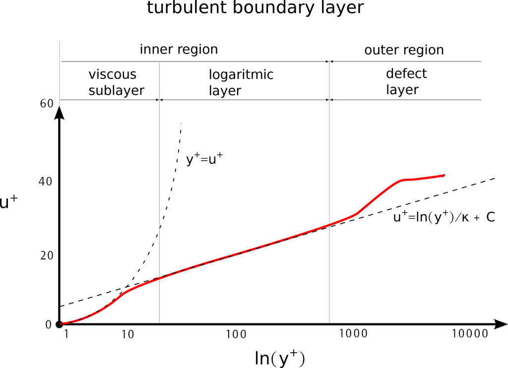
This post will try to consolidate my learnings about the turbulent boundary layers, in particular, the theory leading up to the log-law.
Here, two important assumptions are that of the external flat plate scenario, and that the wall is smooth.
Turbulent Shear Stress
The shear stress is the rate of transportation of momentum per unit area, in the direction normal to that of the flow. From the Navier-Stokes’ x-momentum equation:
\[\rho \frac{\mathrm{d}u}{\mathrm{d}x} = -\frac{\mathrm{\partial}p}{\mathrm{\partial}x} + \frac{\mathrm{\partial}\sigma_{xx}}{\mathrm{\partial}x} + \frac{\mathrm{\partial}\tau_{yx}}{\mathrm{\partial}y} + \frac{\mathrm{\partial}\tau_{zx}}{\mathrm{\partial}z}\]In this particular case, the changes in the quantities of interest in the z-direction is negligible, hence the dominant direction for the shear stress is the y-direction. Also similarly in the RANS[1]:
\[\rho \frac{\mathrm{d}U}{\mathrm{d}x} = -\frac{\mathrm{\partial}\overline{p}}{\mathrm{\partial}x} + \mu\nabla^2 U - \rho \left[ \frac{\mathrm{\partial}\overline{u^{'}u^{'}}}{\mathrm{\partial}x} + \frac{\mathrm{\partial}\overline{u^{'}v^{'}}}{\mathrm{\partial}y} + \frac{\mathrm{\partial}\overline{u^{'}w^{'}}}{\mathrm{\partial}z} \right] + \rho g_x\]Rearranging,
\[\rho \frac{\mathrm{d}U}{\mathrm{d}x} = -\frac{\mathrm{\partial}\overline{p}}{\mathrm{\partial}x} + \rho g_x + \frac{\mathrm{\partial}}{\mathrm{\partial}x} \left( \mu\frac{\mathrm{\partial}U}{\mathrm{\partial}x} - \rho \overline{u^{'}} \overline{u^{'}} \right) + \frac{\mathrm{\partial}}{\mathrm{\partial}y} \left( \mu\frac{\mathrm{\partial}U}{\mathrm{\partial}y} - \rho \overline{u^{'}} \overline{v^{'}} \right) + \frac{\mathrm{\partial}}{\mathrm{\partial}z} \left( \mu\frac{\mathrm{\partial}U}{\mathrm{\partial}z} - \rho \overline{u^{'}} \overline{w^{'}} \right)\]The equation is of the form \(\mathrm{Inertia} = \mathrm{Pressure Gradient} + \mathrm{Body Force} + \mathrm{Turbulent Stresses}\)
The first one in the Turbulent stress terms is the normal stress component, while the remaining two are the shear stresses. The Turbulent Kinetic Energy is associated with the Reynolds Normal Stresses.
These terms are called Turbulent “stresses” because they come in the stress term of the Navier Stokes equations.
The total shear is, hence,
\[\tau = \mu \frac{\mathrm{\partial}U}{\mathrm{\partial}y} - \rho u' v' = \tau_{lam} + \tau_{turb}\]Regions in the Turbulent Boundary Layer
At about \(y < 0.1 \delta\), Laminar/Viscous shear dominates. This inner layer velocity is given by:
\[\begin{equation} u_{\mathrm{inner}} = f\left( y, \tau, \rho, \underline{\mu} \right) \label{eq:1} \end{equation}\]And the outer layer:
\[\begin{equation} u_{\mathrm{outer}} = f\left( y, \tau, \rho, \underline{U_{\mathrm{inf}}}, \underline{\delta} \right) \label{eq:2} \end{equation}\]- Notice that the inner layer is dependent on viscosity and is independent of the free-stream velocity or the boundary layer thickness. Hence it is called the viscous layer
- The outer layer is independent of viscosity, since it is at a sufficient distance away from the wall.
At \(y < 0.1\delta\), \(\tau = \tau_{wall}\)
By dimensional analysis, the shear stress has dimensions of \([\mathrm{density}] * [\mathrm{velocity}]^2\)
Hence, a velocity \(u_{\tau}\) is defined such that
\[\tau = \rho u_{\tau}^2\]where, \(u_{\tau}\) is the Friction Velocity
This velocity is used for non-dimensionalising. [2]
\[u^+ = \frac{U}{u_{\tau}} \ \ \ \mathrm{and} \ \ \ y^+ = \frac{yu_{\tau}}{\nu}\]where \(y^+\) is like a local Reynolds number. A measure of viscous and turbulent transport at different distances from the wall[3].
Law of the wall (Prandtl, 1925)
- Near the wall, the velocity profile is independent of the boundary layer thickness, or the external flow. It is almost purely a viscous effect, a universal function.
- It forms the first layer within the inner layer, within the range of approximately \(y < 0.1\delta\)
Mathematically, equation \eqref{eq:1} can be re-writtten as:
\[u = f_w\left( y, u_{\tau}, \underline{\mu} \right)\]Non-dimensionalising,
\[\begin{equation} U^+ = f_w\left( y^+ \right) \label{eq:3} \end{equation}\]The non-dimensional velocity profile is dependent on \(y^+\) ONLY
\(f_w\) is a UNIVERSAL function
Outer Layer (von-Kármán, 1930)
Mathematically, equation \eqref{eq:2} can be re-written as:
\[u = f\left( y, u_{\tau}, \underline{U_{\mathrm{inf}}}, \underline{\delta} \right)\]Non-dimensionalising, the velocity profile is conveniently written as [4]
\[\frac{U_{\mathrm{inf}} - u}{u_{\tau}} = F\left( \frac{y}{\delta} \right) = F(\eta)\] \[\begin{equation} U_{\mathrm{inf}}^{+} - U^+ = F(\eta) \label{eq:4} \end{equation}\]\(F\) is not a universal function, and depends on the particular type of flow, due to its dependence on \(\eta\), which varies with the boundary layer thickness as well.
Overlap Layer: The Log-Law (C. B. Millikan, 1937)
Millkan noted that, for a smooth transition from the inner layer to outer layer, the velocity profile[5] HAS to be logarithmic. Introducing \(\delta^+ = \delta u_{\tau} / \nu\), so that \(\eta = y/\delta = y^+/\delta^+\)
Adding equations \eqref{eq:3} and \eqref{eq:4}, [6]
\[\begin{equation} U_{\mathrm{inf}}^+\left( \delta^+ \right) = f_w\left( \eta \delta^+ \right) + F\left( \eta \right) \label{eq:5} \end{equation}\]For a function (\(f_w\)) which is dependent on two variables (\(\eta\) and \(\delta^+\)), to be sum of two different functions (\(U_{\mathrm{inf}}^+\) and \(F\)) which are each dependent on one of the respective dependent variables only (\(\eta\) and \(\delta^+\)), the function (\(f_w\)) HAS to be logarithmic.
It approximately comes under the range \(y<0.3\delta\)
This can be proved mathematically as well.
Deriving the inner layer velocity profile function \(f_w\)
Overlap Layer
Differentiating \eqref{eq:5} with respect to \(\delta^+\)
\[\begin{equation} {U_{\mathrm{inf}}^+}^{'} \left( \delta^+ \right) = \eta f_w^{'} \left(\eta \delta^+ \right) \label{eq:6} \end{equation}\]Differentiating \eqref{eq:6} with respect to \(\eta\)
\[0 = \eta \delta^+ f_w^{"} \left(\eta \delta^+ \right) + f_w^{'} \left(\eta \delta^+ \right)\]Substituting for \(y^+\)
\[0 = y^+ f_w^{"} \left(y^+ \right) + f_w^{'} \left(y^+ \right) = \frac{\mathrm{d}}{\mathrm{d}y^+} \left( y^+ \frac{\mathrm{d}f_w}{\mathrm{d}y^+} \right)\] \[y^+ \frac{\mathrm{d}f_w}{\mathrm{d}y^+} = C_1\] \[f_w = C_1\ln y^+ + C_2\]Through experiments, and from \eqref{eq:3}
\[f_w = U^+ = \frac{1}{\kappa}\ln y^+ + B\]- Typically, the values of \(\kappa\) and \(B\) are 0.41 and 5 respectively
- Except in regions of strong adverse pressure gradients (like in diffusers) this is a good approximation of the turbulent boundary layer velocity profile
Near the wall for the viscous sublayer
Very close to the wall, the turbulence fluctuations are dampened out and the wall shear stress is almost entirely viscous, as mentioned before.
\[\tau = \mu \frac{\mathrm{\partial}U}{\mathrm{\partial}y} \implies U = \frac{\tau y}{\mu}\]Substituting for \(\tau = \rho u_{\tau}^2\),
\[U = \frac{\rho u_{\tau}^2 y}{\mu}\] \[\frac{U}{u_{\tau}} = \frac{\rho u_{\tau} y}{\mu} \implies U^+ = y^+\]Hence, from \eqref{eq:3} it is clear that the function \(f_w = y^+\)
A linear variation of the (non-dimensional) velocity profile with \(y^+\) corresponds to the viscous sublayer of \(y^+<5\)
Limits of the regions
As per Pope (2000), the following are the limits of the regions within the inner layer in terms of \(y^+\)
\[U^+ = f_w \left( y^+ \right) = \begin{cases} y^+ & y^+ < 5 & \text{Viscous Sublayer} \\ \text{-} & 5 < y^+ < 30 & \text{Buffer Layer} \\ \frac{1}{\kappa}\ln y^+ + B & y^+ > 30, \ \ y/\delta < 0.3 & \text{Overlap Log-Layer} \end{cases}\]The outer-layer is sensitive to the mean-flow pressure gradient (and hence, dependent on \(U_{\mathrm{inf}}\) and \(\delta\) as in \eqref{eq:2}), and starts deviating from the log-law anywhere above \(y^+\) of as low as 50, or as high as 350-1000, depending on the scenario.
This should make the cover image quite clear. (The x-axis title should be \(y^+\), on a logarithmic scale)
Notes
[1] Remember that,
\[\overline{u^{'}} = \frac{1}{T}\int_{0}^{T} \left( u - u^{'} \right) \ \mathrm{dt} = \overline{u} - \overline{\overline{u}} = \overline{u} - \overline{u} = 0\]But,
\[\overline{u'}^{2} = \frac{1}{T}\int_{0}^{T} \left( u - \overline{u} \right)^{2} \ \mathrm{dt} = \frac{1}{T} \int_{0}^{T} \left( u^{2} + \overline{u}^{2} - 2u\overline{u} \right) \ \mathrm{dt} \ne 0\][2] One question arises: Why not use the free-stream velocity to non-dimensionalise? Technically, we could, but non-dimensionalising should always be done sensibly, and not just choosing any parameter. In this case, the velocity function to be non-dimensionalised is near the wal, which has very little influence from the free-stream conditions, hence also \(U_{\mathrm{inf}}\). It is more sensible to choose a velocity which is dependent to the wall conditions, or specifically, the wall shear stress. Hence the friction velocity is derived through a rough dimensional analysis from the wall shear stress.
[3] Recollect that low \(y^+\) models are also called low Re models
[4] This equation is called the Velocity-Defect Law
[5] Note that the velocity profile is given by the (“universal”) function \(f_w\) for the “inner-layer” - near the wall and the overlap layer as well. Hence, the function \(f_w\) takes on a different value as it crosses towards the overlap layer, as will be seen further.
[6] The free-stream velocity is an independent variable, and the non-dimensional \(U_{\mathrm{inf}}^+ = U_{\mathrm{inf}}/u_{\tau}\) is dependent only on \(u_{\tau}\) and \(\delta\). Hence, it is conveniently chosen as \(U_{\mathrm{inf}}^+ \left( \delta u_{\tau}/\nu \right) = U_{\mathrm{inf}}^+ \left( \delta^+ \right)\)