Turbulence and its Modeling

Definition of Turbulence

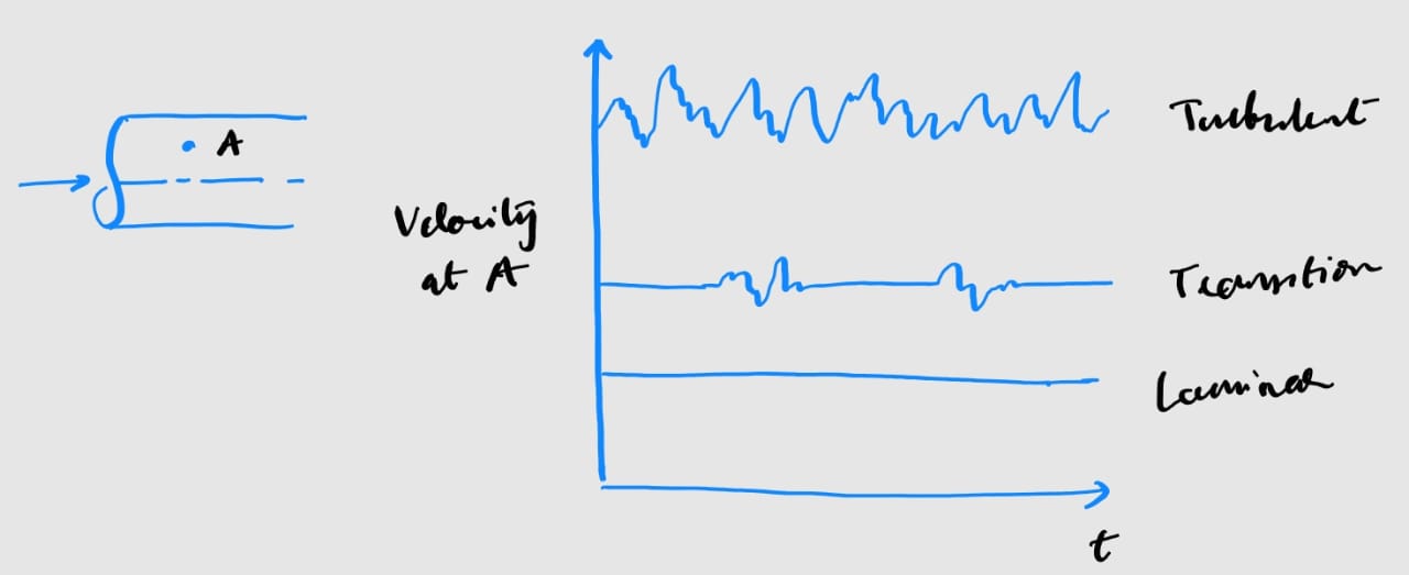
In fluid dynamics, turbulent flow is a fluid motion characterized by chaotic changes in the flow properties. It is in contrast to laminar flow, which occurs when a fluid flows in parallel layers with no disruption between those layers.

Turbulence is a phenomenon which is difficult to define fundamentally. It is often understood by the characteristics which are universally observed in turbulent flows. Some of them are:

• Chaotic; presence of Randomness
• Presence of vortices which are three-dimensional
• Unsteady - not necessarily periodic
• High Reynolds number (not necessarily high speed). Representing (relatively) higher inertial forces
• High mixing (and hence, high diffusivity)
• Dissipating - via an energy cascading mechanism.

Energy Cascading

Turbulence is characterized by eddies. Eddies are turbulent motions localised within a region, and each eddy can be characterized by a Reynolds Number. The larger eddies have higher Re, and take time to dissipate (since viscous effect - which is crucial for higher (molecular) dissipation - is negligible due to high Re).

The energy-cascading mechanism states that the “Large-eddies” dissipates energy to smaller eddies, and further on till the very small eddy with low Reynolds number and high enough viscosity (so that energy is dissipated by viscous effects). It is best described by the rhyming verse by Lewis F. Richardson -

Big whorls have little whorls that feed on their velocity, And little whorls have lesser whorls and so on to viscosity.

Turbulence is, hence, a hierarchy of eddy structures. The size of these eddies can range from flow length scale (characteristic length. e.g., pipe diameter for internal flows) right down to the molecular level. A more mathematical description of the energy cascading is provided by Kolmogorov. According to him, the “small” and “large” eddies are defined based on the demarcation scale $L_e = L_o/6$, where $L_o$ is the length scale compared to flow geometry.

Kolmogorov put forth 3 hypotheses as a more mathematical description of the energy cascade:

1. Local Isotropy

At sufficiently high Reynolds Number, small scale motions are statistically isotropic. i.e., As energy passes down the cascade, all information about directionality (“directional dependence”) of eddies are lost. Hence, they take on a universal character independent of flow geometry.

2. First Similarity

At sufficiently high Reynolds Number, the statistics of small scale motions are universal, determined solely by kinematic viscosity and rate of dissipation of specific Turbulent Kinetic Energy ($\epsilon$).

3. Second Similarity

At sufficiently high Reynolds Number , there exists ranges of motion scales where the properties of motion are uniquely determined by only $\epsilon$.

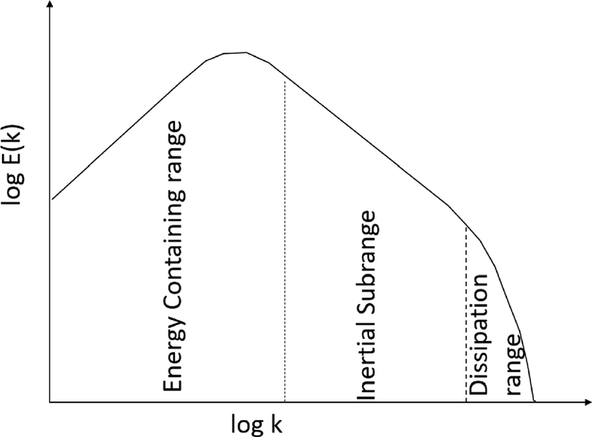Energy vs Wave_number in log-log scale. Wave number is inversely proportional to Length scale

As per the figure above, there are two regions - the Energy Containing Range and the Universal (Equilibrium) Range, demarcated at Length Scale = $L_e$ as defined above. The Universal Range is divided into Inertial Subrange (as per Second Similarity) and the Dissipation Range (as per First Similarity).

Computing Turbulence

As per Kolmogorov, the smallest length and time scales (for dissipation) are defined as (through the aid of simple dimensional anlysis):

\[l_k = \left( \frac{\nu^3}{\epsilon} \right)^{1/4}, \quad t_k = \left( \frac{\nu}{\epsilon} \right)^{1/2} = \frac{l_k^2}{\nu} \left[ \frac{\mathrm{m}^2}{\mathrm{m^2/s}}\right]\]

These values are useful for the optimum mesh settings for capturing turbulence till the lowest length and time scale level. But, this would require extremely fine mesh settings since the time scales can go as low as $10E-6$ seconds, and that requires immense computational power for most engineering problems.

Hence, there is a need to model turbulence. One method to do this is using the RANS approach, where ALL the length scales are mathematicall modeled.

Reynolds Averaging

Due to turbulence, any flow property (say, velocity) at a given point undergoes chaotic fluctuation, as shown in figure below.

Velocity fluctuations due to turbulence at a given point

For any turbulent quantity $\phi$, it can be represented as the summation of the mean of the quantity over a time period, and a fluctuating component. This is called Reynolds Decomposition. Mathematically:

\[\phi = \overline{\phi} + \phi^{\prime}\]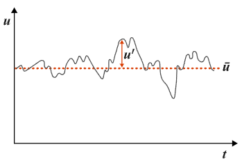

Reynolds Decomposition

By definition, $\overline{\phi^{\prime}} = 0$

Some properties are:

\[\overline{a+b} = \overline{a} + \overline{b}\] \[\overline{c\phi} = c\overline{\phi}\] \[\overline{\nabla \phi} = \nabla \overline{\phi}\] \[\overline{ab} = \overline{\left( \overline{a} + a^{\prime} \right) \left( \overline{b} + b^{\prime} \right) } = \overline{a} \overline{b} + \overline{\overline{a} b^{\prime} } + \overline{a^{\prime} \overline{b} } + \overline{a^{\prime} b^{\prime} } = \overline{a} \overline{b} + \overline{a^{\prime} b^{\prime} }\]

;

The averaging here can be done either over time , or via an ensemble averaging where the experiment is repeated N times and the property at each “cell” averaged. [f1]

When this decomposition - on velocity and pressure - and averaging is applied on the Navier-Stokes equations, it is called Reynolds Averaged Navier-Stokes equations or RANS equations. The derivation for a simple incompressible flow with Newtonian fluid is demonstrated

Reynolds Decomposition on velocity and pressure is:

\[\mathbf{\mathrm{u}} = \overline{\mathbf{\mathrm{u}}} + \mathbf{\mathrm{u}}^{\prime}, \quad p = \overline{p} + p^{\prime}\]

From henceforth, tensor notations are used for easier understanding and representation

Continuity equation

The Continuity equation is:

\[\frac{\partial u_i}{\partial x_i} = 0\]

By Reynolds Averaging about time:

\[\overline{ \frac{\partial u_i}{\partial x_i} } = 0\] \[\frac{\partial \overline{\overline{u_i}} + \overline{u_i^{\prime}}}{\partial x_i} = \frac{\partial \overline{u_i}}{\partial x_i} = 0\]

Which also implies,

\[\frac{\partial u_i}{\partial x_i} = 0 \implies \frac{\partial \overline{u_i}}{\partial x_i} + \frac{\partial u_i^{\prime} }{\partial x_i} = 0 \implies \frac{\partial u_i^{\prime} }{\partial x_i} = 0\]

Momentum equations

The momentum equations are given as:

\[\frac{\partial u_i}{\partial t} + u_j \frac{\partial u_i}{\partial x_j} = -\frac{1}{\rho} \frac{\partial p}{\partial x_i} + \nu \frac{\partial^2 u_i}{\partial x_j^2}\]

Where, as mentioned before, $u_i = \overline{u_i} + u_i^{\prime}$

Taking the Reynolds Average, each term is solved below:

a. Unsteady term

\[\overline{\frac{\partial u_i}{\partial t}} = \frac{\partial \overline{\overline{u_i}}}{\partial t} + \frac{\partial \overline{u_i^{\prime}}}{\partial t} = \frac{\partial \overline{u_i}}{\partial t}\]

b. Advection term

\[u_j \frac{\partial u_i}{\partial x_j} = \overline{u_j} \frac{\partial \overline{u_i}}{\partial x_j} + \overline{u_j} \frac{\partial {u_i^{\prime}}}{\partial x_j} + u_j^{\prime} \frac{\partial \overline{u_i}}{\partial x_j} + u_j^{\prime} \frac{\partial u_i^{\prime}}{\partial x_j}\]

Averaging, the term boils down to

\[\overline{u_j} \frac{\partial \overline{u_i}}{\partial x_j} + \overline{u_j^{\prime}} \frac{\partial \overline{u_i^{\prime}}}{\partial x_j}\]

The final term does not become zero since it involves product of two instantaneous velocity terms. Using chain rule,

\[\overline{u_j^{\prime}} \frac{\partial \overline{u_i^{\prime}}}{\partial x_j} = \frac{\partial \overline{u_i^{\prime}} \overline{u_j^{\prime}} }{\partial x_j} - \overline{u_i^{\prime}} \frac{\partial \overline{u_j^{\prime}}}{\partial x_j} = \frac{\partial \overline{u_i^{\prime}} \overline{u_j^{\prime}} }{\partial x_j}\]

The second term in above equation is zero due to continuity equation.

Hence, the advection term becomes:

\[\overline{u_j} \frac{\partial \overline{u_i}}{\partial x_j} + \frac{\partial \overline{u_i^{\prime}} \overline{u_j^{\prime}} }{\partial x_j}\]

c. Pressure term

\[-\frac{1}{\rho} \frac{\partial \left( \overline{\overline{p}} + \overline{p^{\prime}} \right)}{\partial x_i} = -\frac{1}{\rho} \frac{\partial \overline{p} }{\partial x_i}\]

d. Diffusion Term

\[\overline{\nu \frac{\partial^2 \left( \overline{u_i} + u_i^{\prime} \right)}{\partial x_j^2} } = \nu \frac{\partial^2 \overline{u_i}}{\partial x_j^2}\]

Substituting these terms in the final Reynolds Averaged Momentum equations:

\[\begin{equation} \frac{\partial \overline{u_i}}{\partial t} + \overline{u_j} \frac{\partial \overline{u_i}}{\partial x_j} = -\frac{1}{\rho} \frac{\partial \overline{p} }{\partial x_i} + \nu \frac{\partial^2 \overline{u_i}}{\partial x_j^2} - \frac{\partial \overline{u_i^{\prime}} \overline{u_j^{\prime}} }{\partial x_j} \label{eq:1} \end{equation}\]

The above equation is seemingly similar to the transport equation of mean momentum in the case of laminar flow, with 4 unknowns and 4 equations. But the final term consists of instantaneous velocities, represented in tensor form as:

\[\overline{u_i^{\prime}} \overline{u_j^{\prime}} = \left(\begin{array}{lll} \overline{u^{\prime} u^{\prime}} & \overline{u^{\prime} v^{\prime}} & \overline{u^{\prime} w^{\prime}} \\ \overline{v^{\prime} u^{\prime}} & \overline{v^{\prime} v^{\prime}} & \overline{v^{\prime} w^{\prime}} \\ \overline{w^{\prime} u^{\prime}} & \overline{w^{\prime} v^{\prime}} & \overline{w^{\prime} w^{\prime}}\end{array}\right)\]

This is a symmetric tensor, and is called the Reynolds Stress Tensor.

• “Stress” because it has the same units as (specific) stress ( = [stress/density] )
• “Tensor” because, obviously, it is a tensor

This term contains 6 unknowns, and since separate transport equations are unavailable for these, we have more number of unknowns than the number of equations. This closure problem is called the Turbulence Closure Problem.

In order to solve this, the RST is to be addressed directly or indirectly.

Modeling the Reynolds Stress Tensor

These terms are called moments in statistical theory.

\[\mathrm{O} \left(u^{\prime}*u^{\prime} \right) \to \mathrm{2nd \ order \ moments}\] \[\mathrm{O} \left(u^{\prime}*u^{\prime} * u^{\prime} \right) \to \mathrm{3rd \ order \ moments, \ and \ so \ on}\]

The Closure Problem can be solved using 2 approaches:

1. To model the RST directly -> First Order Closure
2. To develop equations for RST and model those 3rd order moments -> Second Order Closure

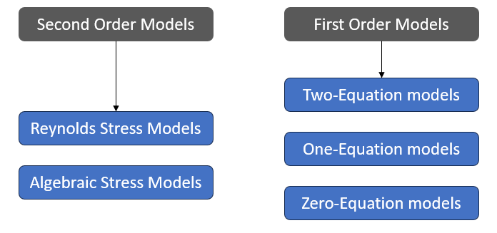Reynolds Averaged Turbulence Models

Each of the schemes has its advantages and disadvantages. Regarding the First-Order Models, they are roughly addressed here.

;

[f1] Note on RANS vs URANS, Time vs Ensemble Averaging

Regarding time vs ensemble averaging

• First of all, the concept of an ensemble average cannot exist in CFD since to perform multiple simulations will take up lot of computational power. Hence, an ensemble average DOES NOT exist explicitly. This is not the distinguishing factor between RANS and URANS.
• There exists something called ergodicity. It is the assumption that the statistical properties of a system (e.g., turbulence) can be obtained from a single realization over a sufficiently long time period. In other words, it is the idea that a point of a moving system, either a dynamical system or a stochastic process, will eventually visit all parts of the space that the system moves in, in a uniform and random sense.
• Hence, in equilibrium systems, time and ensemble averages of physical quantities are equivalent due to the assumption of ergodicity.

Regarding the distinction between RANS and URANS

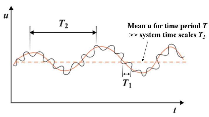
• It can be observed in the final form of RANS (equation $\eqref{eq:1}$) that an unsteady term is present for the mean flow. This term is zero in the case of steady RANS, since the time period used for averaging is much larger, even higher than any time scales present in the simulation. In this case, any variations in the mean flow is also averaged out and a single mean velocity is output (orange dashed line in figure), which is the result obtained after eventual convergence
• But say there exists turbulent structures which has a significant time period ($T_2$), and we choose a time period $T_1$ as the period for averaging such that $T_1 < T_2$. In this case, these turbulent structures are also captured within the simulation (thick orange line in figure). But choosing a higher averaging time period would result in a almost constant mean velocity, which does not change with time, and hence is a steady simulation.
• In the case of steady RANS, the unsteady term is similarly forced to be zero, while in URANS a user-input time period is used to capture the turbulent structures within the frequency of averaging time period.
• Note that $T_1$ still needs to be considerably larger than the largest turbulence (integral) time scale, as URANS can only give a time averaged mean value for the velocity field, not solving turbulence (Altair help)

Reynolds Averaging - URANS vs RANS

Also worth noting the comment from this website:

URANS extends the RANS approach by allowing for time-dependent changes in the flow field, making it capable of capturing unsteady phenomena. It still utilizes the Reynolds averaging of the Navier-Stokes equations but does not average the flow in time as strictly as RANS. This means URANS can model larger-scale transient flow features and oscillatory behaviors, which are typical in many practical engineering systems, such as vortex shedding from building corners. While URANS improves upon RANS in terms of capturing unsteadiness, it still employs eddy-viscosity models that may not adequately resolve finer turbulent structures