The Fourier Transform
I had started my journey in acoustics as a CFD engineer quite recently. And while I had solved quite a lot of complex problems on aero-acoustics (more posts on them later), I encountered a huge obstacle when I passed on to the validation part: the presence of several microphone data having the acoustic pressure vs time, but absolutely no information on processing it. So I started my investigations on the same. The deeper I went in (“how, “why”), the further I understood, and even more I was fascinated. And then I hit the fundamental concept of this order-establishing, entropy-reversing methodology. The Fourier Transform.
We all had this in our curriculum during our graduation, and like most students, I paid no heed to it. This topic was just another one to rote, and even though I understood some parts of the concept here and there, I never could truly appreciate the true glory of this concept. Yes, it has its limitations (which, too, I had stumbled on gradually as I was progressing in my journey of this investigation), but to state the limitations makes me feel like a vain judge. Also, partly it is true that the teacher often acts as the brain-eyes for the students…
Anyway, here I am not writing to teach: for the audience of this blog is the vacuum, me. This is my submission as a self-storage note. Most of the content here is formulated thanks to the extremely intelligent Brant Sanderson, who runs the 3B1B channel. The video of his, which I had gone through, I shall link at the end of this post. [1]
So, this post is sort of a memory-jogger for me, based on which I will write several more, which are all my personal experiments for a deeper understanding of the Fourier Transform.
Why is a pure-tone signal Sinusoidal?
Is it merely a coincidence that a pure tonal signal is sinusoidal in nature? Or is it a mathematical construct? To put it simply, it is ofcourse a “human construct” in the sense that mathematics is, as a language, an “invention”. But the concept itself is not; it is a fundamental law of the universe.
In nature, a sinusoidal wave isn’t just a shape we invented; it is the physical consequence of stability. When any physical system is pushed slightly out of equilibrium - whether it’s an acoustic pressure perturbation in a fluid, a pendulum, or a spring - the universe tries to pull it back. In almost all stable systems, for small displacements, this restoring force is directly proportional to the displacement itself. We know this as Hooke’s Law: $F = -kx$.
By Newton’s second law, $F=ma$, which is the second derivative of position. This gives us the fundamental differential equation governing nearly all natural vibrations:
\[m\frac{d^2x}{dt^2} = -kx\] \[\frac{d^2x}{dt^2} + \frac{k}{m}x = \frac{d^2x}{dt^2} + \omega^2x = 0\]where $\omega$ is the angular frequency of the system. This ODE represents a Simple Harmonic Motion, and the only mathematical solution to this - the purest form of a vibration in the universe - is a sinusoidal function.
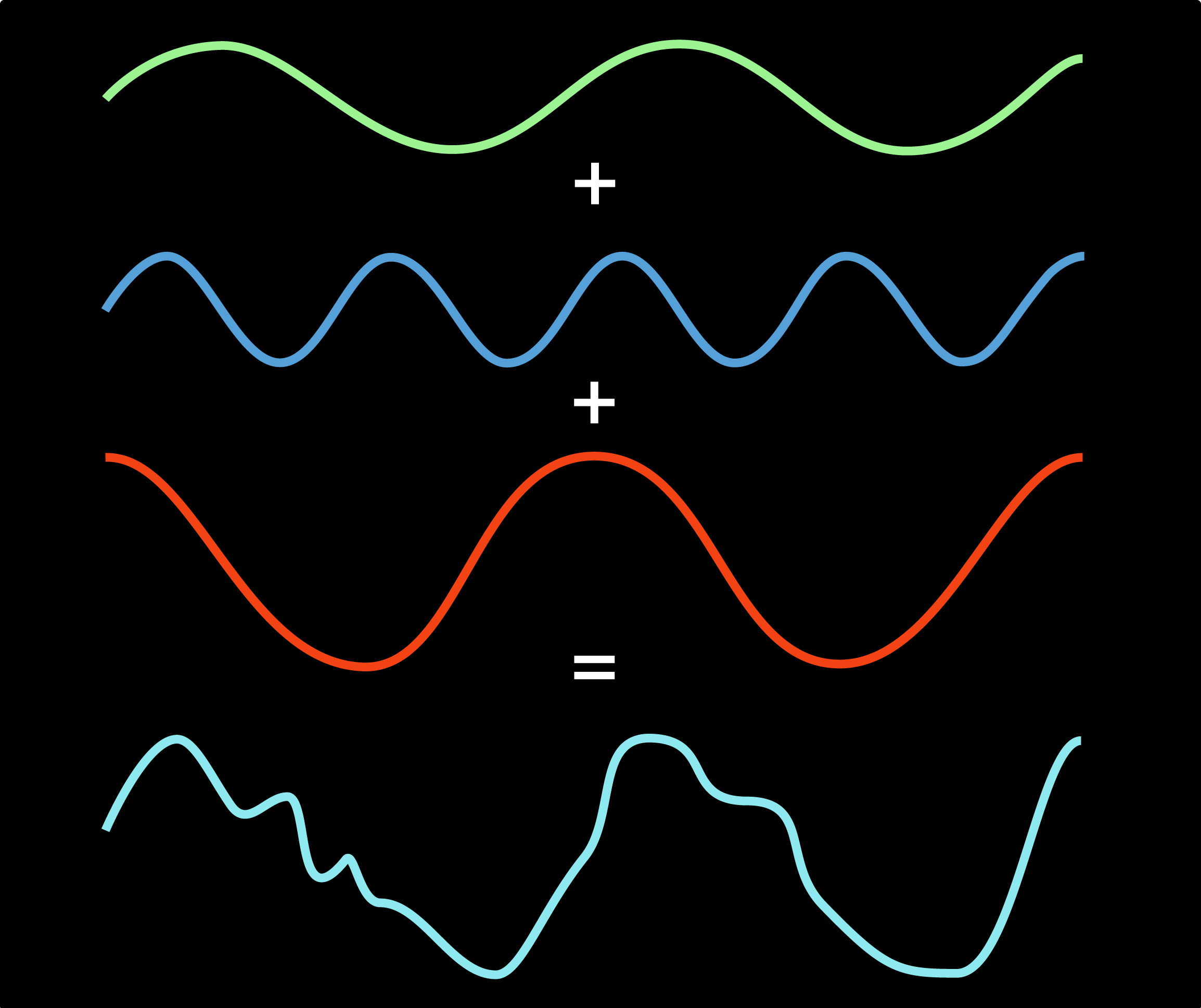
In this direction, it was Joseph Fourier who proved that any periodic signal, no matter how jagged or complex, can be represented as a sum of pure sine and cosine waves.
Relevance of Fourier Transform
So, a signal (say, an acoustic wave) is hence defined by an amplitude and a frequency. In acoustics, the amplitude is the Pressure - how it varies with respect to time - and the frequency is how many times the pressure oscillates around a mean per second. In terms of human senses, this translates as the “loudness” and the pitch of a sound, respectively.
A sound wave which has 500 oscillations per second will have a lower pitch than a wave with 1000 oscillations per second (Hertz). You can play around with many sound signals on this website, although be careful when using headphones.
A combination of waves with two different frequencies would, hence, look more complex and not like a simple sinusoidal wave. For example, in the figure below, there are two sinusoidal waves (green and orange) of different “pitches”. A combination of the two (white dotted) gives a wave which is quite unlike its sinusoidal parents. This wave is just a simple algebraic sum of the pressure amplitudes for each time instance of both the pure frequency waves.
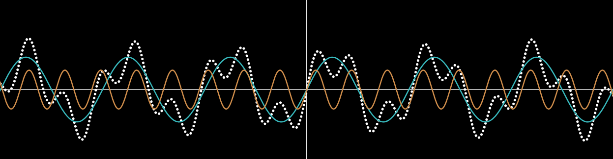
Now, if you place a microphone to record this audio, it cannot distinguish between the two frequencies.. it only records the summation as the final output. Now consider a much more complex signal, in which case the final output could be a combination of MANY sinusoidal waves. How do we get the spectral (frequency-wise) information from this, then?
This is the “entropy-reversal” I was referring to. It is like extracting the ingredients of a mixture of solutions. It is like extracting the individual colours after mixing them all together.
The Circle
The core idea of the Fourier Transform is to wrap a given signal around a circle. Refer to the animation below for a 3Hz wave being “wrapped” in a circle. Let us call this the “wrapping plane” (WP)
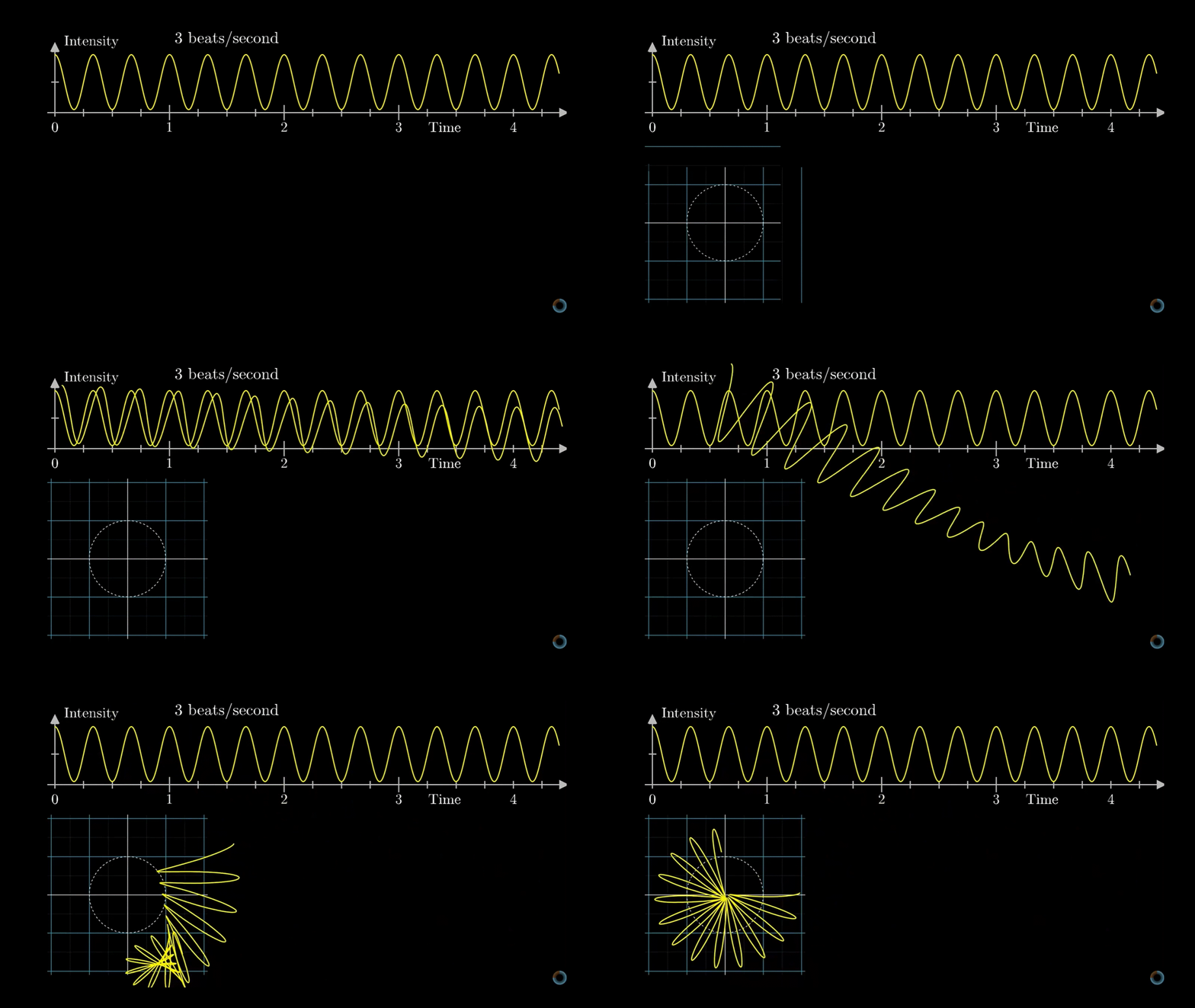 Wrapping of a wave around the “Wrapping Plane”
Of course, the “wrapping” can have its own frequency, defined by how much of the signal is wrapped in one revolution along the WP. If we go around one revolution of the WP in one second, the “wrapping frequency” is 1Hz. Consequently, this means that for a (say) 5Hz signal, the 5 oscillations spread across one second of signal are mapped along the WP, with the amplitudes (positive and negative) defining the curve trajectory when the wrapping is taking place.
This may be a little difficult to understand, but I have made this cute little interactive tool below to visualise this. See that when you have the “wrapping frequency” as 2Hz (i.e., 2 revolutions in one second), half of the 5 oscillations (i.e., in this case of a sine wave, 3 peaks and 2 troughs) is mapped in one revolution in the WP.
Original Signal: f(t) = sin(2π(5)t)
Wrapped Signal (Clockwise)
One can notice the beautiful patterns which are formed when tracing this wave along a circle at various frequencies…
Now, a natural curiosity arises. What happens when the “wrapping frequency” is equal to the frequency of the signal itself?
Below is an animation of a 5Hz wave wrapped at different frequencies. A red point represents the centroid of the shape at any given wrapping frequency instant. Notice that the centroid is almost always very close to the origin any way we wrap the 5Hz signal around the circle. But as the wrapping frequency arrives at 5Hz, the shape unusually changes and the centroid has an eccentric value w.r.t the origin.
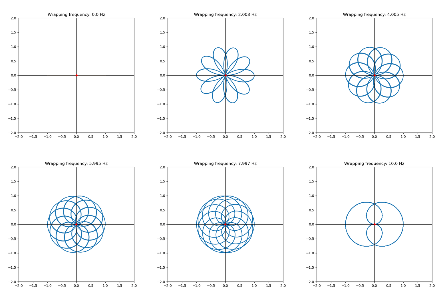 Wrapping of a 5Hz wave at various Wrapping Frequencies
If I plot the distance of this centroid (for now, I will consider the distance and will come to the x and y coordinates later) for different wrapping frequencies, you’ll see a spike for the 5Hz value.
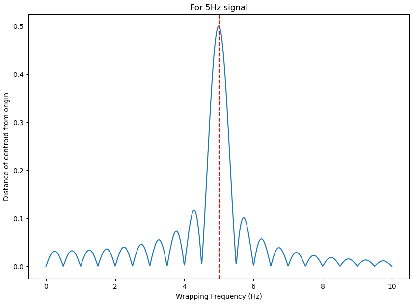 Distance of centroid from origin for a 5Hz signal
This peak is observed only when the frequency of the wave matches the wrapping frequency. Also, notice that the peak value of this centroid distance is exactly 0.5 : which is HALF of the value of the maximum amplitude of the original wave (More on this in a later post): be it a 20Hz signal or a 20,000Hz signal.
Now, what happens if the signal is no longer a pure single-frequency signal, but a combination of multiple frequencies?. Consider this combined signal containing two sine waves: 10Hz of 0.7 amplitude and 6Hz of 1.3 amplitude.
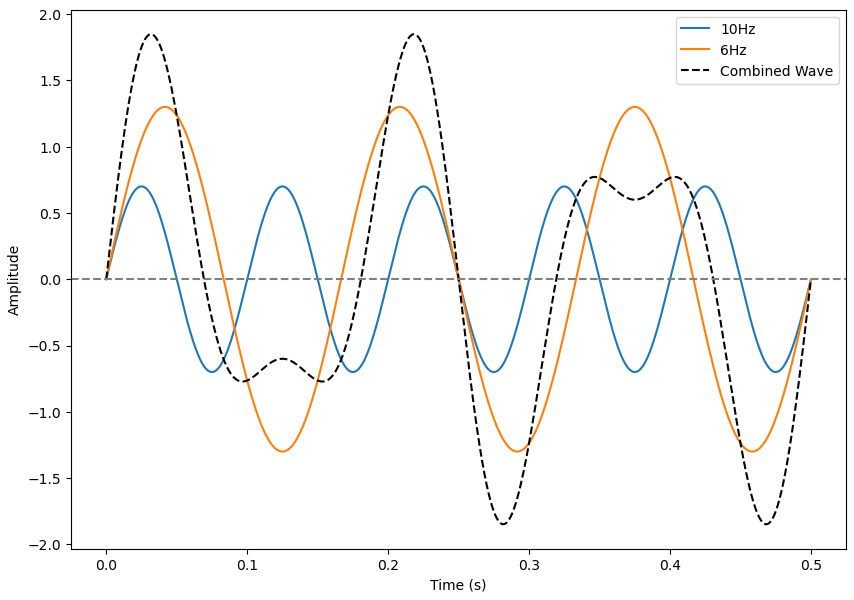 Composite sine wave containing 2 frequencies
Let us “wrap” this combined wave around the circle at different frequencies:
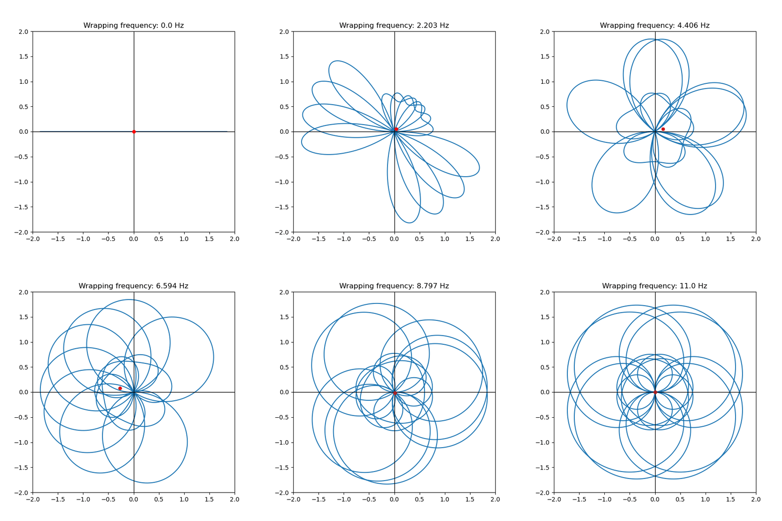 Wrapping of the composite sine wave at various Wrapping Frequencies
Again, plotting the centroid distance from the origin:
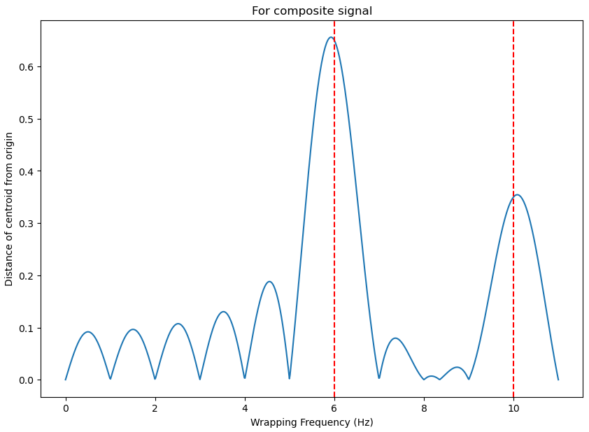 Distance of centroid from origin for a composite signal
Two things can be observed:
- Peak of centroid distance (i.e., eccentricity) at wrapping frequencies of 6Hz and 10Hz: which are the frequencies the composite signal is comprised of!
- The “distance” of the centroid is exactly half of the amplitudes of the individual component waves, i.e., 0.35 for 10Hz and 0.65 for the 6Hz waves, respectively!
Again, more on the magnitude of the peaks later, but look at the elegance of the methodology in identifying the individual component frequencies and also their amplitudes in a given composite wave!
Mathematical Formulation
Euler’s Equation
Before we go into the mathematical formulation, it is important to understand WHAT the x and y coordinates of this “wrapping plane” are. Here, the WP is represented in a complex plane, where the x-axis is the Real axis and the y-axis is the “Imaginary” axis. In a complex plane, the multiplication of any quantity by the imaginary complex number $i$ results in the quantity being rotated 90 degrees counterclockwise. This is obvious if you consider an example: multiply the number “$5$” by $i$, and you get $5i$, which lies on the +y axis in the complex plane.
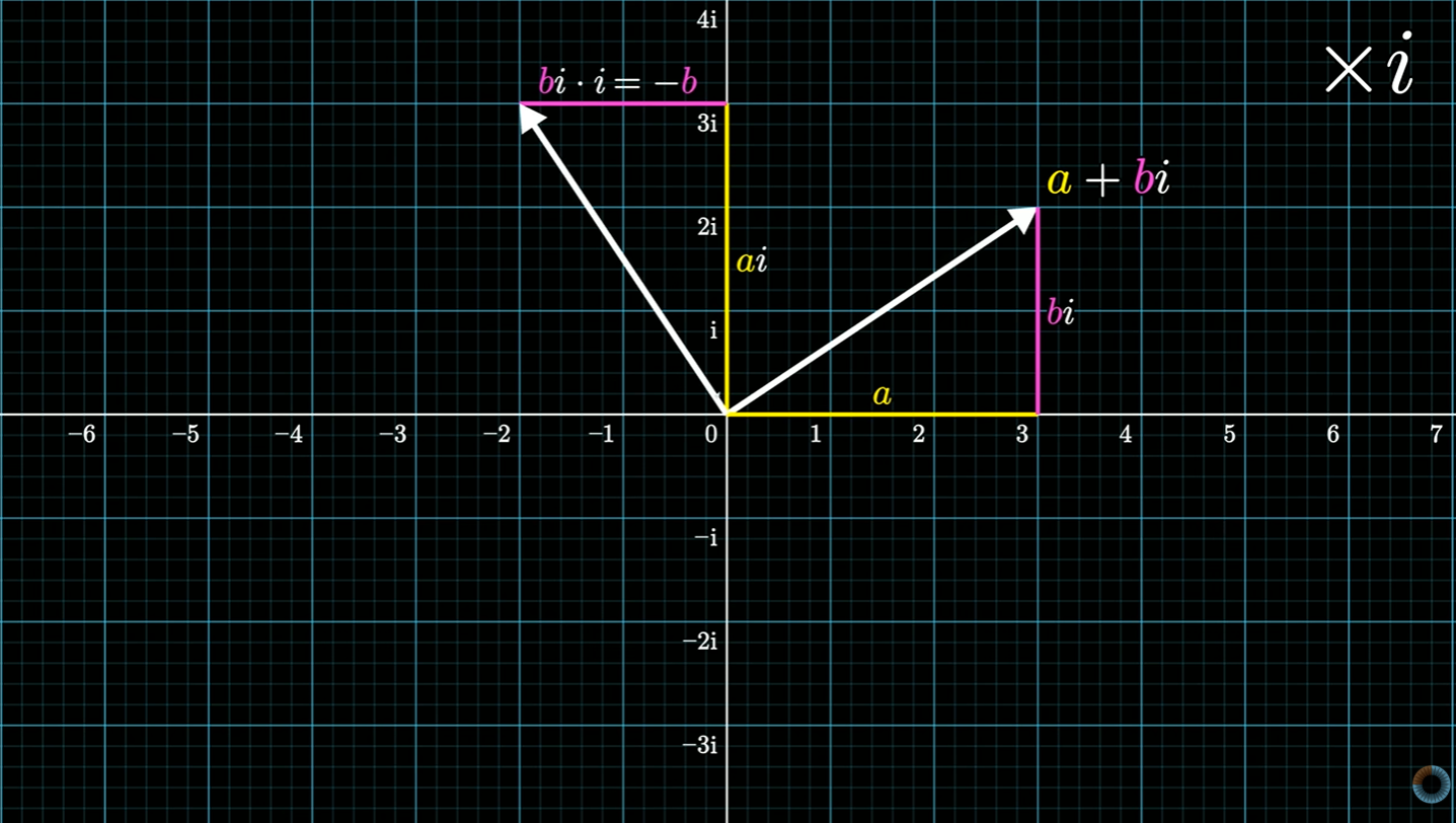 Complex Plane multiplication
To take this a step further, let us bring in the number “$\mathrm{e}$”.
The unique character of this number is: the “natural” exponential function $\mathrm{e}^x$ (the “x” here has nothing to do with the “x” coordinate) is its own derivative. It means that the slope of the curve at any given point is equal to the function value at that point. In other words, the velocity vector of a position vector function $\mathrm{e}^x$ is the function itself. When the exponent factor is a negative number (say $\mathrm{e}^{-0.5x}$), then this represents decay, and if it is a positive number, it represents exponential growth.
What if the exponent factor is $i$? i.e., $\mathrm{e}^{ix}$?
From the chain rule, we have the velocity vector:
\[\frac{d}{dx}\mathrm{e}^{ix} = i\mathrm{e}^{ix}\]Thus, the tendency of a body at a given point in the complex plane having a position vector $\mathrm{e}^{ix}$ is to move perpendicular to its current position. This means that the “engine” of this position vector (i.e., the velocity) pushes it towards a 90degree rotation at every instance. The only mathematical possibility for this body to move is in a counter-clockwise CIRCLE in the complex plane, such that the velocity vector is always perpendicular to the position vector.
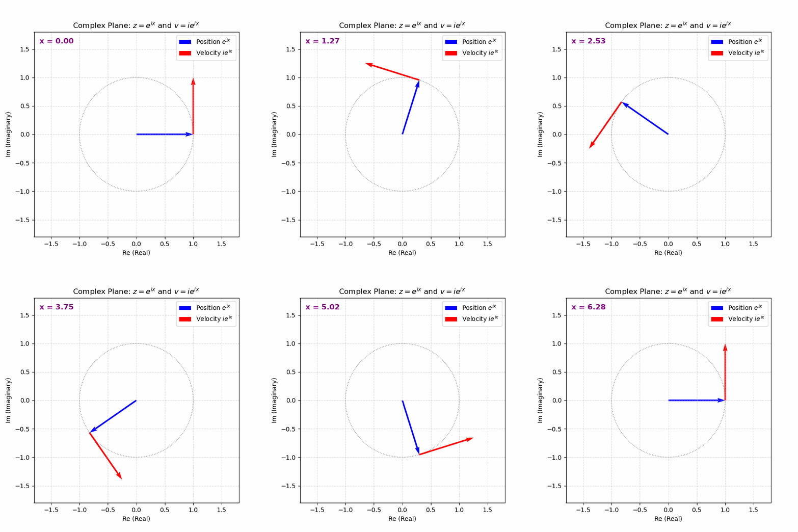 Complex Plane Rotation
The initial condition for this position vector is (at $x$ = 0): $\mathrm{e}^{i0} = 1$. For a full 360-degree rotation, the value of the position vector is back to one, and for a 180-degree rotation, it is -1.
We know the circumference of a unit circle is $2\pi$, hence we get the famous and elegant formula:
\[\mathrm{e}^{i\pi} = -1\]Using the above understandings, one can easily arrive at Euler’s equation, which establishes a fundamental relationship between the trigonometric functions and the complex exponential function. It states that for any real number x:
\[\mathrm{e}^{ix} = \mathrm{cos}x + i\mathrm{sin}x\]Mathematical formulation of the Fourier Transform
Now we will proceed to understand the mathematical expression of the Fourier Transform, step by step.
(1) As understood earlier, one FULL rotation along the unit circle in a complex plane is represented by:
\[\mathrm{e}^{2\pi i}\](2) If one wants to measure this with respect to the time progression, the equation becomes
\[\mathrm{e}^{2\pi it}\](3) The above equation represents rotation along the unit circle in the complex plane w.r.t time, at a rate of one revolution per second. If you want to regulate this “speed” of revolution, then multiply the exponent by a “frequency” term (which is the “Wrapping” frequency). Thus,
\[\mathrm{e}^{2\pi ift}\](4) In the Fourier Transform, the convention is to wrap a given signal Clockwise. Since the above formulae represent Counter-Clockwise rotation, we shall add a negative sign in the exponent.
\[\mathrm{e}^{-2\pi ift}\](5) Till now, the position vector is only tracing a circle. If we want to incorporate the mapping of the signal amplitudes into this circle, then simply multiply by the signal amplitude, which we can define as a function $g(t)$. Hence, we can modify the equation to
\[g(t)\mathrm{e}^{-2\pi ift}\](6) The above equation still only represents the “wrapped curve” in the graph, and not the centroid itself, which, as we established earlier, is the identifier of the individual frequencies and their amplitudes present in the signal wave.
If you construct the wave as a set of many points which are sampled very close together, then - after wrapping the wave around a circle at any particular (“wrapping”) frequency $f$ - the centroid can be computed as simply the average of all the points collected together. Mathematically,
\[\frac{1}{N}\sum_{k=1}^{N}g(t)\mathrm{e}^{-2\pi ift}\](7) For these points placed infinitesimally close together, we convert the discrete nature of the above equation to integrals:
\[\frac{1}{t_2 - t_1}\int_{t_1}^{t_2}g(t)\mathrm{e}^{-2\pi ift}\]The actual Fourier Transform is only the integral part, and does not contain the normalising factor of the time delta:
\[G(f) = \int_{t_1}^{t_2}g(t)\mathrm{e}^{-2\pi ift}\]This means that, if the signal contains a particular frequency wave, then the Fourier Transform of this signal is scaled according to the time this particular composite signal has run.
This Fourier transform, let us call it the “Standard” FT, represents the TOTAL energy of a particular frequency signal in the waveform.
While this is useful, many solvers - especially for aero-acoustics - retain the “Normalisation denominator”. If a signal is a continuous hum (like fan noise, or flow over an ORVM), the Standard FT can take up massive values based on the total time of recording, since it represents the TOTAL energy of the signal.
\[G(f) = \frac{1}{t_2 - t_1}\int_{t_1}^{t_2}g(t)\mathrm{e}^{-2\pi ift}\]By dividing by $(t_2 - t_1)$, the Average Amplitude (or power) of that frequency during that specific time window is being calculated. In short, the Standard FT outputs units of $[Value].[Time]$, while the “Normalised” FT outputs units of $[Value]$.
In real-world engineering problems, we want the magnitude of the Fourier result to relate directly to the physical oscillation. If you have a sine wave with a peak pressure of $10\text{ Pa}$, a normalised transform will give you a peak at that frequency representing $10\text{ Pa}$. Without that $t_2 - t_1$ normalization, the value would grow larger the longer you ran your simulation, which wouldn’t make physical sense.
Footnotes
[2] The codes for images and animations generated by self, and even further, are consolidated here.
[3] Link for self-investigations into the Fourier Transform. (1)